Notes on 4.12 Data collection and reliability
Learning objectives
Describe how to design a valid data collection method, such as a questionnaire, using unbiased, structured and precise questions.
Identify biased, personal, unstructured and imprecise questions and suggest improvements.
Select the variables and data that are relevant to a research question, and justify the choice.
Explain the difference between reliability and validity.
Describe the test-retest and parallel forms methods for checking reliability, and use a correlation coefficient to judge reliability.
Describe content validity and criterion-related validity, and use a correlation coefficient to judge criterion-related validity.
Justify the choice of categories for a chi-squared table, combining classes so that every expected frequency is greater than 5.
Determine the number of degrees of freedom in a chi-squared goodness of fit test when parameters are estimated from the data.
Explain why a single significant result among many tests should be treated with caution.
Introduction
Every statistical conclusion is only as good as the data behind it. A hypothesis test on badly collected data gives a precise-looking p-value that answers the wrong question, and a correlation between two badly measured quantities says little about the quantities themselves. Before any calculation, an investigator has to decide what to measure, how to ask for it, which data to keep, and how to check that the measuring instrument gives consistent and meaningful results. After the data are in, grouping them for a chi-squared test involves further decisions: which classes to use and how many degrees of freedom remain once some features of the model have been taken from the data themselves.
Questionnaires used in medicine, education and recruitment are checked in exactly these ways. A personality test that sorts a person into a different type when they repeat it a few weeks later, or an entrance test whose scores bear no relation to later performance, may be popular and still be of little use as a measurement.
Designing valid data collection methods
Subtopic 4.1, Collecting data and sampling, deals with who is asked: the population, the sample and the sampling method, and the bias that a poor sample introduces. A well-chosen sample can still produce poor data if the questions put to it are badly designed. Data collection design deals with what is asked and how.
Surveys and questionnaires
A survey collects information from members of a sample, often through a fixed list of questions. The list of questions is the measuring instrument, in the same way that a thermometer is the instrument for temperature.
A questionnaire has to be designed so that every respondent understands each question in the same way, answers it honestly, and gives an answer that can be recorded and analysed. When this fails, the answers measure something other than what the investigator intended. The faults fall into a small number of types, each with its own name.
Biased and unbiased questions
The wording of a question can push respondents towards one answer. "Does the dangerous junction outside the school need traffic lights?" calls the junction dangerous before the respondent has given a view, and invites agreement.
Bias in a question can come from loaded words ("dangerous", "wasteful", "fair"), from a statement of what others think, from offering more positive answer options than negative ones, or from a yes/no format that invites agreement. An unbiased version states the issue neutrally and offers balanced options: "Should traffic lights be installed at the junction outside the school? Yes / No / No opinion."
A real example of neutral wording being tested comes from the 2016 United Kingdom referendum on membership of the European Union. The Bill first proposed the question "Should the United Kingdom remain a member of the European Union?" with the answers Yes and No. After testing it with members of the public, the Electoral Commission found the wording was not seen as balanced and recommended a question naming both outcomes, with the answers "Remain a member of the European Union" and "Leave the European Union", which it judged the most neutral of the options it had tested.
Source: Wikipedia, "European Union Referendum Act 2015", citing the Electoral Commission's assessment of September 2015.
Personal questions
Some questions ask for information that people may prefer to keep private: income, weight, health, illegal behaviour, school grades. Respondents may refuse to answer, round their answer, or give a socially acceptable answer instead of the true one.
Personal questions cannot always be avoided, since sometimes the sensitive variable is the one being studied. Their effect can be reduced by keeping the questionnaire anonymous, by explaining how the data will be used, and by asking for a range instead of an exact value ("Annual income: under $30,000 / $30,000 to $59,999 / $60,000 or more"). Removing anonymity to "check" answers usually makes the problem worse, because fewer people answer honestly or at all.
Structured and unstructured questions
Questions differ in how much freedom the respondent has in answering.
The two types serve different purposes. Structured questions give data that can be counted, tabulated and tested straight away, so they suit large samples and statistical analysis; their weakness is that the answer options may not include what the respondent wants to say. Unstructured questions collect richer and unexpected information, which suits a small pilot study before the main survey, but the answers have to be read and grouped by hand before any analysis, and two people grouping them may disagree.
Structured question | Unstructured question | |
|---|---|---|
Answers | chosen from fixed options | in the respondent's own words |
Analysis | quick: counts in each category | slow: answers must be read and grouped |
Suits | large samples, statistical tests | pilot studies, exploring new ideas |
Weakness | options may not fit every respondent | grouping is subjective; hard to compare |
Precise questions
A question must mean the same thing to every respondent. "Exercise regularly: yes / no" is answered "yes" by someone who walks to school and by someone who trains every day, because "regularly" and "exercise" are not defined.
A precise version of the exercise question states what counts and over what period: "Number of days in the last 7 days with at least 30 minutes of physical activity causing hard breathing: 0 / 1–2 / 3–4 / 5–7." Precision also means asking one thing at a time. "Is the library quiet and well stocked?" is a double question: a respondent who finds it quiet but poorly stocked has no correct answer.
Selecting relevant variables and data
A data set downloaded from a statistics office, a sports database or a school's records may contain dozens of variables for each individual. Analysing all of them is neither possible nor useful. The first step is to state the research question precisely, and the second is to decide which variables bear on it.
For the question "Does the amount of sleep a student gets affect their reaction time?", the relevant variables are hours of sleep and a measured reaction time. Variables that could also affect reaction time, such as age or caffeine intake, are relevant too, because they may need to be controlled or recorded. Eye colour and favourite subject are not relevant and should not be collected: every extra variable lengthens the questionnaire, lowers the response rate and creates more opportunities for chance patterns.
Choosing relevant and appropriate data
Once the variables are chosen, the investigator decides which observations to keep. The data analysed must match the population named in the research question, the time period it refers to and the conditions under which the comparison is fair.
The right population. A question about adult women's heights needs data on adult women only, not a file of all ages.
The right time period. Average house prices from 2010 say little about prices now.
Comparable conditions. Comparing marathon times from a flat course with times from a hilly course compares the courses as much as the runners.
The right type and level of detail. A chi-squared test needs counts in categories; a correlation needs paired numerical data; ranks are enough for Spearman's .
Clean data. Values that are impossible (a height of 17 m), duplicated or missing are dealt with before analysis. An outlier is removed only for a stated reason, such as a recording error or an individual outside the population, never simply because it weakens the result.
Many variables and multiple testing
A large data set tempts an investigator to test every variable against every other and report whatever turns out to be significant. This is a misuse of hypothesis testing. At the 5% significance level, a test of a true null hypothesis gives a significant result with probability 0.05, so if enough tests are carried out, some will be significant by chance alone.
If independent tests are each carried out at the 5% level and every null hypothesis is true, the number of significant results is . The probability of at least one significant result is found from the complement.
Number of tests | 1 | 5 | 10 | 20 | 25 | 50 |
|---|---|---|---|---|---|---|
0.050 | 0.226 | 0.401 | 0.642 | 0.723 | 0.923 |
Probability of at least one significant result at the 5% level when every null hypothesis is true and the tests are independent.
The probability rises quickly: with 20 tests a chance "discovery" is more likely than not. A single significant result found among many tests should therefore be treated as a suggestion to investigate with new data, not as a finding. The honest approach is to choose the relevant variables and the hypotheses before looking at the data.
Reliability and validity
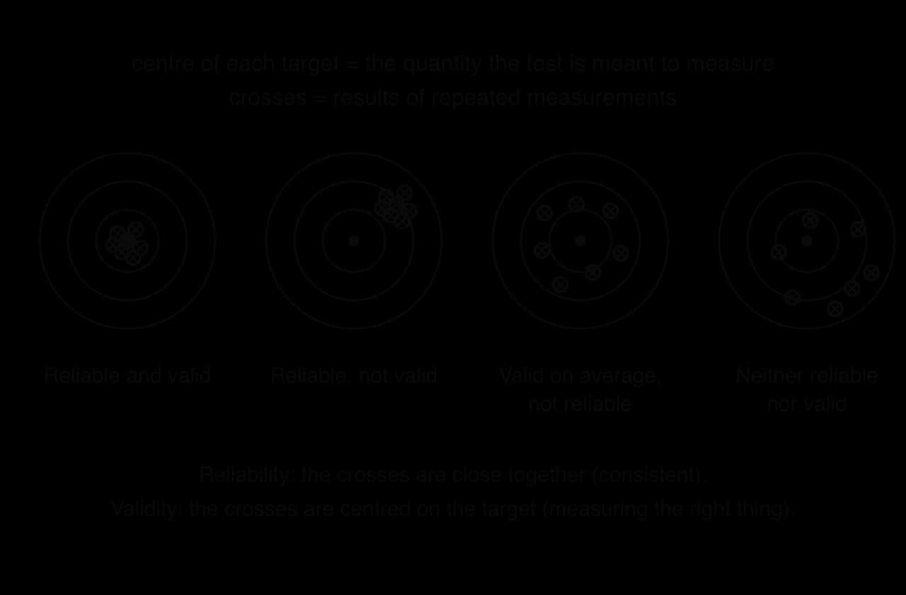
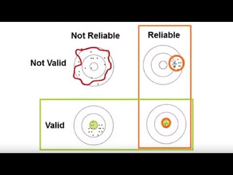
Any measuring instrument, whether it is a bathroom scale, a reading test or a personality questionnaire, is judged in two separate ways. One is whether it gives the same result when the same thing is measured again; the other is whether it measures the thing it claims to measure. The first is reliability, met in subtopic 4.1 as the trustworthiness of a data source; in the measurement sense, a reliable test gives consistent results when it is repeated under the same conditions. The second is validity.
This meaning is different from the validity of a model in subtopic 2.6, which asks whether a mathematical model describes a real situation well enough for its purpose. A test can be reliable without being valid: a bathroom scale that always reads 2 kg too heavy gives consistent readings, but every reading is 2 kg above the true mass. A test that is not reliable cannot be valid in any useful way, because a measurement that changes at random from one occasion to the next cannot be measuring a fixed quantity accurately.
The four targets in the diagram of reliability and validity show the four combinations. Each cross is the result of one measurement, and the centre of the target is the true value of the quantity being measured.
Measuring agreement with a correlation coefficient
Each method of checking reliability or validity produces two sets of scores for the same individuals: two sittings of a test, two versions of a test, or a test and a later outcome. The strength of the agreement between the two sets is measured with a correlation coefficient: Pearson's product-moment correlation coefficient for numerical scores with a linear relationship (subtopic 4.4), or Spearman's rank correlation coefficient for ranks or a relationship that is monotonic but not linear (subtopic 4.10). A value close to 1 means strong agreement, so the test is judged reliable (or valid); a value well below 1 means weak agreement. There is no fixed cut-off. Values above about 0.8 are usually described as showing good reliability, and the judgement is stated with the value quoted: "
Test-retest reliability
The most direct check of consistency is to give the same test twice.
The gap between the two sittings needs care. If it is too short, people remember their answers and simply repeat them, which makes the test look more reliable than it is. If it is too long, the quantity being measured may genuinely change (a student's reading ability improves over a term), which makes a reliable test look unreliable. A gap of a week or a few weeks is typical for a test of a stable characteristic.
Eight students take a reading test and then take the same test again two weeks later. The graph of the second score against the first, with the line on which the two scores are equal, shows how closely the scores agree.
Student | A | B | C | D | E | F | G | H |
|---|---|---|---|---|---|---|---|---|
First sitting | 34 | 41 | 28 | 45 | 38 | 30 | 47 | 36 |
Second sitting | 36 | 39 | 31 | 44 | 40 | 27 | 46 | 38 |
Scores out of 50 on two sittings of a reading test (hypothetical data).
Entering the two lists into the GDC's linear regression (or two-variable statistics) function gives . The value is close to 1, so the reading test shows good test-retest reliability. The correlation coefficient measures agreement in the pattern of the scores and ignores any constant difference between them. If every student scored exactly 5 marks more on the second sitting, would still be 1.
Case study: the Myers–Briggs Type Indicator
The Myers–Briggs Type Indicator is a widely used personality questionnaire that sorts each person into one of 16 "types". If personality types are stable, a person who takes it twice a few weeks apart should get the same type both times. Studies of its test-retest reliability have found that between 39% and 76% of respondents obtain a different type classification when they retake it after only five weeks.
Source: Wikipedia, "Myers–Briggs Type Indicator", 2025, summarising published reliability studies.
A measurement that changes for a large fraction of people over five weeks cannot be measuring a fixed characteristic accurately, whatever else its merits. Popularity and reliability are separate questions: an instrument used by millions of people still needs evidence that it gives consistent results. The case also shows a weakness of sorting into categories. A person whose score lies close to the boundary between two types can move across the boundary with a small change in score, so a categorical result can look less reliable than the underlying scores.
Parallel forms reliability
The memory problem of test-retest reliability can be avoided by writing two different versions of the test.
Organisations that run language and entrance tests use parallel forms all the time, since each sitting needs a new version of the same standard. The method has its own disadvantages. Writing two genuinely equivalent versions takes time and expertise, and if one version turns out to be harder, the correlation can still be high (the order of the candidates is kept) while the scores are not comparable. The two versions may also be given at almost the same time, which reduces the effect of genuine change in the people being tested.
Test-retest | Parallel forms | |
|---|---|---|
What is given | the same test twice | two equivalent versions |
Main advantage | only one test to write | no memory of earlier answers |
Main disadvantage | memory and practice effects; real change over the gap | hard to make the versions equally difficult; time-consuming to write two |
Measured by | or between the two sets of scores |
Parallel forms checks are also used for attitude questionnaires, where the same people complete two versions with differently worded items a few days apart.
Member | 1 | 2 | 3 | 4 | 5 | 6 | 7 |
|---|---|---|---|---|---|---|---|
Version A | 3.2 | 4.1 | 2.5 | 3.8 | 4.6 | 2.9 | 3.5 |
Version B | 3.4 | 3.9 | 2.8 | 3.3 | 4.4 | 3.1 | 3.9 |
Average item scores (1 to 5) of seven club members on two versions of a motivation questionnaire (hypothetical data).
In the motivation example, the GDC value is . A strong correlation shows that the two versions put the members in nearly the same order. Whether the two versions are equally hard to agree with is a separate question, answered by comparing their means.
Content validity
Reliability concerns consistency only, and leaves open what is being measured. A spelling test can be very reliable and still be a poor test of a student's ability to write an essay. Validity is checked in different ways, two of which have names.
A final test in a mathematics course has good content validity if its questions cover every topic of the course in proportion to the teaching time, and poor content validity if two-thirds of the marks come from one topic. A questionnaire on "well-being" that asks only about sleep has poor content validity, however consistent its answers. Content validity is a matter of judgement with no correlation coefficient attached. The evidence is the opinion of people who know the subject well, often recorded by comparing the test item by item with a list of what should be covered.
Criterion-related validity
The second method compares the test with an independent measure of the same quantity, called the criterion.
A new 10-minute screening test for reading difficulty could be compared with a long, established assessment given in the same week (concurrent validity). A university entrance test could be compared with the same students' results at the end of their first year (predictive validity). In both cases, a strong positive correlation means the test ranks people in much the same way as the criterion, so it is a valid measure of what the criterion measures.
The choice of criterion matters. If the criterion is itself unreliable or measures something slightly different, a low correlation may say more about the criterion than about the test. Predictive validity can be checked only on the people who were selected, since those who scored low were never admitted and have no later results, so the data cover only part of the range and the correlation is often weaker than the true relationship.
Student | A | B | C | D | E | F | G | H | I | J |
|---|---|---|---|---|---|---|---|---|---|---|
Test score | 62 | 75 | 58 | 81 | 70 | 66 | 88 | 54 | 73 | 79 |
First-year grade | 5 | 6 | 4 | 6 | 5 | 6 | 7 | 4 | 5 | 7 |
Entrance test scores and first-year grades of 10 students (hypothetical data).
 YouTube
Improving reliability and validity
The two properties are improved in different ways, and a criticism of a study should say which one it concerns.
Reliability improves with a larger sample, a higher response rate, standard conditions and clear instructions for every respondent, structured and precise questions, and checks such as a test-retest or parallel forms study.
Validity improves when the questions measure the quantity itself instead of a stand-in for it (self-reported happiness is not the same as happiness; self-reported exercise is not the same as measured activity), when the sample is random so that it represents the population named in the question, when the content covers every aspect of the quantity, and when the results are checked against a criterion.
Categorising numerical data for a chi-squared test
The chi-squared goodness of fit test and the test for independence of subtopic 4.11 compare counts in categories. When the data are numerical (heights, waiting times, numbers of goals), they have to be grouped into categories before the test, and the choice of categories is part of the method. It affects the expected frequencies, the degrees of freedom and, in the end, the conclusion.
Why expected frequencies must exceed 5
The statistic
follows the chi-squared distribution only approximately, and the approximation is poor when some expected frequencies are small. Dividing by a small makes a single extra observation produce a large contribution: with , observing 3 instead of 1 adds
Combining classes
When some expected frequencies are 5 or less, neighbouring classes are merged until every expected frequency exceeds 5.
The rules for combining follow from what the test is meant to do.
Calculate all the expected frequencies first, before merging anything. The decision depends on expected frequencies, never on observed ones.
Merge a class with expected frequency of 5 or less into its neighbour, usually towards the centre of the distribution. For numerical data, adjacent classes keep the order of the values: merging "0 goals" with "4 goals" would make a meaningless category.
Merge only as much as needed. Each merge removes a category and therefore a degree of freedom, and makes the test less able to detect a poor fit in that part of the distribution.
Combine the observed frequencies of the same classes and recompute the expected frequencies' totals, so that both still add up to the total frequency.
The tails of a distribution are where small expected frequencies usually appear, so the last few classes (or the first few) are the ones combined. An open-ended last class such as "4 or more" is needed anyway, so that the probabilities of all the classes add up to 1.
Justifying the choice of categories
A grouping has to be justified whenever it is chosen. A good justification refers to the following points.
Every expected frequency is greater than 5, so the chi-squared approximation is valid.
Classes are adjacent and do not overlap, and together they cover every possible value.
There are enough classes left to compare the shape of the data with the model, which needs at least three or four classes; with only two classes the test compares a single proportion.
The class boundaries are natural for the context (whole numbers of goals, 5-minute intervals of time) and were chosen before the observed frequencies were seen, so they were not picked to make the result look better.
For continuous data, the classes are intervals such as . The expected frequency of each class is the total frequency multiplied by the probability of the interval under the model, with the first and last classes open-ended.
Degrees of freedom when parameters are estimated
In subtopic 4.11 every model was fully specified before the data were collected: a fair die, a 9 : 3 : 3 : 1 ratio, or a normal distribution with a stated mean and standard deviation. The degrees of freedom were the number of categories minus 1. Often, though, the question is only whether the data follow some Poisson distribution, or some normal distribution, and the parameter values are not known in advance. They have to be taken from the data.
Why each estimated parameter costs one degree of freedom
The degrees of freedom count how many of the frequencies can vary freely once the constraints are fixed. In any goodness of fit test, the expected frequencies are made to add up to the observed total, which is one constraint: once frequencies are known, the last is fixed.
Estimating a parameter adds another constraint. When the mean of a Poisson model is taken from the data, the model's expected frequencies are forced to have the same mean as the observed frequencies. The model has been adjusted to match the data in one more respect, so the observed and expected frequencies are automatically closer than they would be for a model chosen in advance, and tends to be smaller. Reducing the degrees of freedom by one moves the critical value down to compensate, and the same reasoning applies to every further parameter estimated from the data.
The table shows how the rule applies to the distributions in the course.
Model | Parameters estimated from the data | Degrees of freedom with classes |
|---|---|---|
Fully given (equal, ratio, stated parameters) | none | |
Binomial , |
Here is the number of classes after* combining.*
In a binomial model the number of trials is part of the experiment (5 seeds in each packet, 6 bulbs in each box), so it is known and is never estimated. A parameter that the question gives, for example a mean "from historical records", is not estimated from the data and costs no degree of freedom.
Estimating the parameters
The estimates come from the sample, with technology.
Poisson mean : the sample mean of the data, from the GDC's one-variable statistics with the values in one list and the frequencies in another. The Poisson distribution is taught in subtopic 4.17.
Binomial probability : the sample mean divided by the number of trials,
The estimated value is then treated as the parameter for the expected frequencies: each class probability comes from the model with that parameter, multiplied by the total frequency.
Case study: deaths from horse kicks in the Prussian army
In 1898 the Russian-German statistician Ladislaus von Bortkiewicz published counts of soldiers killed by horse kicks in 10 corps of the Prussian army over 20 years. Each corps in each year is one observation, giving 200 corps-years. Deaths were rare, unpredictable and independent of each other, the kind of event a Poisson distribution describes.
Deaths in a corps-year | 0 | 1 | 2 | 3 | 4 |
|---|---|---|---|---|---|
Number of corps-years | 109 | 65 | 22 | 3 | 1 |
Source: L. von Bortkiewicz (1898), via Andrews and Herzberg (1985), dataset HorseKicks in the R package vcd (Rdatasets).
No mean was known in advance, so it is estimated from the data. The total number of deaths is
The variance of the data is
Under the number of deaths in a corps-year follows . The expected frequencies are
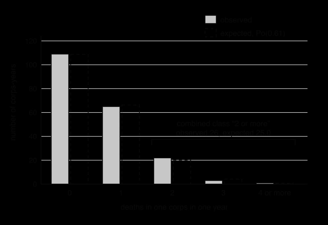
Deaths | 0 | 1 | 2 | 3 | 4 or more |
|---|---|---|---|---|---|
Observed | 109 | 65 | 22 | 3 | 1 |
Expected | 108.67 | 66.29 | 20.22 | 4.11 | 0.71 |
The last two expected frequencies are less than 5. Merging "3" and "4 or more" gives , still not greater than 5, so "2" has to join them as well: the class "2 or more" has expected frequency and observed frequency
Deaths | 0 | 1 | 2 or more |
|---|---|---|---|
Observed | 109 | 65 | 26 |
Expected | 108.67 | 66.29 | 25.04 |
After combining there are 3 classes, and one parameter (the mean) was estimated, so
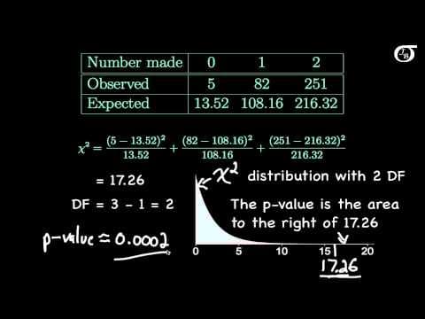
The GDC's goodness of fit test with these lists and gives and p-value
The case shows the price of combining. The data originally had five classes; after merging, only three remain, and estimating the mean leaves a single degree of freedom. A test with one degree of freedom compares the data with the model in only one respect, so it has little power to detect a poor fit in the tail. Collecting more data, so that more classes have large enough expected frequencies, is the way to test the tail properly.
GDC procedure for a goodness of fit test with estimated parameters
Enter the values and their observed frequencies in two lists, and use one-variable statistics to find (and for a normal model).
Find the probability of each class from the model with the estimated parameters, using the distribution functions (Poisson, binomial or normal probability and cumulative probability). Use the complement for the open-ended last class.
Multiply each probability by the total frequency to get the expected frequencies, and write them down, usually to 2 or more decimal places.
Combine classes until every expected frequency is greater than 5, adding observed and expected frequencies of the merged classes.
Enter the combined observed and expected frequencies in two lists and run the goodness of fit test, typing in the reduced degrees of freedom by hand: on a TI-84 Plus CE,
STAT→TESTS→
Complaints | 0 | 1 | 2 | 3 | 4 | 5 | 6 |
|---|---|---|---|---|---|---|---|
Days | 18 | 35 | 32 | 20 | 9 | 4 | 2 |
Customer complaints per day over 120 days (hypothetical data).
The merge in the complaints example stopped as soon as every expected frequency exceeded 5. Merging from 4 upwards would also satisfy the rule, but it would remove another class and another degree of freedom for no gain. Any grouping of adjacent classes that meets the rule can be justified, and the smallest merge keeps the most information.
 YouTube
A binomial model with p estimated
In a binomial goodness of fit test, the number of trials is fixed by the situation and only may be unknown. Estimating it from the data uses the fact that the mean of is .
Faulty bulbs | 0 | 1 | 2 | 3 | 4 | 5 | 6 |
|---|---|---|---|---|---|---|---|
Boxes | 30 | 38 | 22 | 7 | 2 | 1 | 0 |
Faulty bulbs in 100 boxes of 6 (hypothetical data).
A normal model with mean and standard deviation estimated
When neither nor is known, both are estimated, and two extra degrees of freedom are lost.
Length (mm) |
|---|
Lengths of 200 leaves (hypothetical data).
The degrees of freedom change the conclusion's strength noticeably. With the same statistic, 7.00, the wrong value gives a p-value of 0.321 instead of 0.136. In a borderline case the wrong choice can reverse the decision, so the degrees of freedom deserve as much care as the statistic itself.
Exam focus
Data collection, reliability and validity appear mostly as short parts of a long Paper 3 question that reviews a whole study, and occasionally as a short Paper 1 question. Typical parts ask you to state the name of a test for reliability or validity (1 mark), describe a criticism of a study's reliability or validity (1 mark each, with a reason that links to the property), suggest an improvement, calculate or between two sets of scores and hence determine whether the test is reliable or valid (2 marks: the value close to 1, then the conclusion), or find the probability of at least one significant result among many tests. Questions on categorising data and degrees of freedom appear inside goodness of fit questions on Papers 1, 2 and 3: they ask you to find expected frequencies, explain why classes must be combined, write down the degrees of freedom and carry out the test. Write the combined table,
Number of flaws | 0 | 1 | 2 | 3 | 4 | 5 |
|---|---|---|---|---|---|---|
Number of sheets | 40 | 52 | 33 | 16 | 7 | 2 |
Flaws in 150 sheets of glass (hypothetical data).
In part (g) the expected frequency for "4 or more" under is 5.07, just above 5, so the same five classes can be kept. The test gives and p-value 0.350, so the claimed model is not rejected either. Both models are consistent with the data; the data cannot distinguish between a mean of 1.2 and a mean of 1.36 with this sample size.
The other common question shape reviews a whole investigation: a survey with a low response rate, a self-reported variable, a sample from one place, a quota or convenience sample described in the stem. Each criticism needs a reason tied to bias, reliability or validity. Naming the sampling method (subtopic 4.1) is often a part of the same question.
Practice questions
A questionnaire contains the question "How often do you eat fast food?" with the options "Never / Sometimes / Often". Identify one weakness of this question and write down an improved version. [2]
Explain the difference between a structured question and an unstructured question, giving one advantage of each. [3]
Six athletes do a balance test twice, one week apart. Their scores are 12, 15, 9, 18, 14, 11 on the first occasion and 13, 14, 10, 17, 15, 9 on the second, in the same order. (a) State the name of this test for reliability. [1] (b) Find Pearson's product-moment correlation coefficient. [2] (c) Hence comment on the reliability of the balance test. [2]
A company's new aptitude test is given to 8 trainees. Their scores are 48, 61, 55, 72, 66, 58, 80, 52, and their performance ratings by a manager six months later are 3, 5, 3, 6, 4, 4, 7, 2, in the same order. (a) State the name of this type of validity. [1] (b) Find Spearman's rank correlation coefficient. [3] (c) Hence comment on the validity of the aptitude test. [2]
A researcher carries out 12 independent hypothesis tests at the 5% significance level. In fact every null hypothesis is true. Find the probability that at least one test gives a significant result. [3]
The number of goals in 80 matches is to be tested against the model . The expected frequencies are 10.83, 21.65, 21.65, 14.44, 7.22 and 4.21 for 0, 1, 2, 3, 4 and "5 or more" goals. (a) Explain which classes should be combined. [2] (b) Write down the number of degrees of freedom. [1] (c) Write down the number of degrees of freedom if, instead, the mean had been estimated from the 80 matches and the same classes used. [1]
Write down the number of degrees of freedom in each goodness of fit test. (a) A normal model with given mean and estimated standard deviation, 6 classes after combining. [1] (b) A normal model with both parameters estimated, 8 classes before combining and 6 after. [1] (c) A binomial model with estimated, 5 classes, none combined. [1]
In 120 families with 3 children, the numbers of girls are: 0 girls: 18 families, 1 girl: 45, 2 girls: 40, 3 girls: 17. (a) Find an estimate of the probability that a child is a girl. [2] (b) Find the expected frequencies under a binomial model. [2] (c) Test, at the 5% significance level, whether a binomial model is suitable. [4]
A survey of a town's residents is carried out by emailing a link to members of a local walking club. The survey asks "How many hours of exercise did you do last week?" Describe one criticism of the validity of the survey's estimate of the exercise done by the town's residents. [2]
Answers
"Sometimes" and "often" are imprecise (they mean different things to different people) and there is no time frame. Improved: "In the last 7 days, on how many days did you eat food from a fast-food outlet? 0 / 1–2 / 3–4 / 5 or more."
Structured: fixed answer options, the same for everyone; quick to count and analyse. Unstructured: answered in the respondent's own words; collects detail and unexpected answers (useful in a pilot study).
(a) Test-retest. (b) . (c) is close to 1, so the balance test is reliable.
(a) Criterion-related (predictive) validity. (b) Ranks of scores 1, 5, 3, 7, 6, 4, 8, 2; ranks of ratings 2.5, 6, 2.5, 7, 4.5, 4.5, 8, 1;
Summary
A questionnaire should use unbiased, precise and, for analysis, structured questions with consistent, exhaustive and non-overlapping options; personal questions need anonymity or ranges.
Choose the relevant variables and data before analysis, matching the population, time period and conditions of the research question; remove outliers only for a stated reason.
With independent tests at 5% and every true,
Self-check
- To do:
I can identify a biased, personal, unstructured or imprecise question and rewrite it.
- To do:
I can write structured answer options that are consistent, exhaustive and non-overlapping.
- To do:
I can choose the variables and data relevant to a research question and justify leaving others out.
- To do:
I can calculate and explain why one significant result among many tests is doubtful.
- To do:
I can explain the difference between reliability and validity, with an example of a reliable but invalid test.
- To do:
I can name and describe the test-retest and parallel forms methods, with a disadvantage of each.
- To do:
I can name and describe content validity and criterion-related validity.
- To do: