4.11 Hypothesis testing

Set up null and alternative hypotheses, use p-values and significance levels, and carry out chi-squared tests for independence and goodness of fit and the pooled two-sample t-test, with conclusions in context.

IB Mathematics: Applications and Interpretation
Part of 4 Statistics and probability
SL and HL

Key terms introduced here

Each is in the Maths AI glossary, with every other term in the subject.

Alternative hypothesis: The statement, written $\mathrm{H}_1$ , that is accepted if the null hypothesis is rejected; it describes a difference, an association or a departure from a model.
Chi-squared distribution: The continuous probability distribution, taking only non-negative values, that the chi-squared statistic follows when the null hypothesis is true; its shape is set by the number of degrees of freedom.
Chi-squared goodness of fit test: A test of whether observed frequencies in a set of categories are consistent with the frequencies predicted by a stated distribution.
Chi-squared test for independence: A test of whether two categorical variables are independent in a population, using the observed frequencies in a contingency table.
Contingency table: A table of observed frequencies that classifies each member of a sample by two categorical variables, one for the rows and one for the columns.
Critical value: The boundary value of a test statistic for a given significance level; a test statistic beyond the critical value leads to rejecting the null hypothesis.
Degrees of freedom: The number of frequencies in a chi-squared calculation that can vary freely once the totals are fixed, written $\nu$ (or df).
Expected frequency: The number of observations predicted for a category if the null hypothesis were true, written $f_e$ ; it is the total frequency multiplied by the probability of the category under the null hypothesis.
Hypothesis test: A procedure that uses sample data to decide whether there is enough evidence to reject a stated claim about a population.
Null hypothesis: The statement of no difference, no association or no change from a model, written $\mathrm{H}_0$ , that is assumed true while a hypothesis test is carried out.
Observed frequency: The number of observations actually recorded in a category of a sample, written $f_o$ .
One-tailed test: A test whose alternative hypothesis states the direction of the difference from the value in the null hypothesis.
p-value: The probability, assuming the null hypothesis is true, of obtaining a test statistic at least as extreme as the one calculated from the sample.
Significance level: The threshold probability, chosen before a test is carried out, below which the p-value leads to rejecting the null hypothesis; it equals the probability of rejecting the null hypothesis when it is in fact true.
Statistically significant: Describes a result whose p-value is less than the chosen significance level, so that the null hypothesis is rejected at that level.
t-test: A test of whether the means of two populations are equal, using independent random samples from each; the pooled two-sample t-test assumes both populations are normally distributed with equal variances.
Test statistic: A single value calculated from the sample data that measures how far the data are from what the null hypothesis predicts.
Two-tailed test: A test whose alternative hypothesis states only that a parameter differs from the value in the null hypothesis, in either direction.

Notes on 4.11 Hypothesis testing

50 min readLast reviewed 15 Oct 2026

Learning objectives

State a null hypothesis and an alternative hypothesis for a test, as an equation, an inequality or in words.
Explain the meaning of a significance level and a p-value, and use them to decide whether to reject the null hypothesis.
Calculate expected frequencies from observed frequencies, for a contingency table and for a given model.
Determine the number of degrees of freedom for a chi-squared test.
Perform a chi-squared test for independence, using a p-value or a given critical value.
Perform a chi-squared goodness of fit test for a given distribution, including a normal model with given mean and standard deviation.
Perform a pooled two-sample t-test to compare the means of two populations, using technology.
Distinguish between one-tailed and two-tailed tests and choose the right one from the claim being tested.
Interpret the result of a test in context, and state the assumptions a test depends on.

Introduction

A hypothesis test is a way of deciding, from a sample, whether the evidence is strong enough to doubt a claim about a whole population. A drug company wants to know whether a new treatment lowers blood pressure more than the old one; a geneticist wants to know whether offspring appear in the ratio a theory predicts; a school wants to know whether students' choice of transport depends on their year group. In each case the sample results differ from what the claim predicts, and the question is whether the difference is larger than chance variation alone would produce.

Every hypothesis test follows the same logic: assume a cautious claim of "no effect", measure how far the data are from what that claim predicts, and find the probability of a discrepancy at least that large if the claim were true. A small probability counts as evidence against the claim. Three tests are built on it: two chi-squared tests for counts in categories and a t-test for comparing two means.

The logic of a hypothesis test

A claim about a population, such as "the die is fair" or "the two fertilisers give the same mean height", cannot usually be checked by examining the whole population. Instead a random sample is taken, and the sample results are compared with what the claim predicts. Because samples vary by chance, the results never match the prediction exactly, even when the claim is true. A hypothesis test replaces the vague question "is the difference big?" with a precise calculation of the probability of a difference at least this big if the claim is true.

The method resembles a criminal trial. The defendant is presumed innocent, and the verdict "guilty" is reached only if the evidence makes innocence hard to believe. In the same way, a test starts by presuming the cautious claim of "no difference" and rejects it only if the data would be very surprising under that claim. A verdict of "not guilty" means only that the evidence was not strong enough to convict, and a test that does not reject its starting claim has the same limited meaning.

Null and alternative hypotheses

Every test compares two competing statements about the population. The first is the default position, which is assumed true while the test is carried out. It always contains the idea of equality, no difference, no association or "the model fits", because only then can the probabilities in the test be calculated.

The second statement is what the investigator suspects might be true instead, and it is accepted only when the data give enough evidence against $\mathrm{H}_0$ .

Hypotheses are statements about populations, not about the samples. The sample means of two groups of plants are known exactly once the plants are measured, so there is nothing to test about them. The test asks about the population means, written $\mu_1$ and $\mu_2$ : the mean heights of all plants that could be grown with each fertiliser. For the same reason, a chi-squared hypothesis concerns two variables in the whole population, not the particular people surveyed.

Hypotheses may be written in symbols (an equation or inequality) or in words, whichever is clearer or whichever a question asks for. The table shows the standard forms for the chi-squared tests and the t-test.

Test	$\mathrm{H}_0$	$\mathrm{H}_1$
Chi-squared test for independence	The two variables are independent	The two variables are not independent
Chi-squared goodness of fit test	The data fit the stated distribution (name it, with any parameters)	The data do not fit the stated distribution
t-test, two-tailed	$\mu_1 = \mu_2$	$\mu_1 \ne \mu_2$
t-test, one-tailed	$\mu_1 = \mu_2$	$\mu_1 > \mu_2$ (or $\mu_1 < \mu_2$ )

For a chi-squared test for independence, the word "independent" has the meaning of independent events from subtopic 4.6: knowing the category of one variable does not change the probabilities for the other. Words such as "related", "correlated", "linked" or "influences" describe something different (correlation applies to numerical data in subtopic 4.4) and should not be used. "Not associated" is an acceptable alternative to "independent".

State suitable null and alternative hypotheses for each investigation.

(a) A researcher wants to know whether a person's favourite type of music depends on their age group.

(b) A games designer wants to test whether a spinner with five equal sectors lands on each sector equally often.

Show the solution

(a) This is a question about two categorical variables, so a chi-squared test for independence is used.

$\mathrm{H}_0$ : favourite type of music and age group are independent.

$\mathrm{H}_1$ : favourite type of music and age group are not independent.

(b) The spinner is compared with a model (each sector has probability $\frac{1}{5}$ ), so this is a goodness of fit test.

$\mathrm{H}_0$ : the spinner lands on each sector with probability $\frac{1}{5}$ (the spinner is fair).

$\mathrm{H}_1$ : the spinner does not land on each sector with probability $\frac{1}{5}$ .

(c) Two population means are compared. Let $\mu_A$ and $\mu_B$ be the population mean egg weights for hens fed diet A and diet B.

$\mathrm{H}_0$ : $\mu_A = \mu_B$

$\mathrm{H}_1$ : $\mu_A > \mu_B$

The biologist's belief has a direction ("heavier"), so the alternative hypothesis uses $>$ .

Significance levels and p-values

Once the hypotheses are stated, the data are summarised by a single number that measures how far they are from what $\mathrm{H}_0$ predicts. Large values (or, for some tests, values far from zero in either direction) count against $\mathrm{H}_0$ .

The key quantity in a test is the probability of getting data at least as far from $\mathrm{H}_0$ as the data actually observed, calculated on the assumption that $\mathrm{H}_0$ is true. If this probability is very small, then either a rare event has happened or $\mathrm{H}_0$ is wrong, and the test chooses the second explanation.

A p-value is a probability, so it always lies between 0 and 1. A small p-value means that the data would be surprising if $\mathrm{H}_0$ were true, and so gives evidence against $\mathrm{H}_0$ . A large p-value means that the data are quite consistent with $\mathrm{H}_0$ . How small is "small enough" is decided before the data are collected, by choosing a threshold.

The choice of level reflects how costly a wrong rejection would be. A 1% level demands stronger evidence than a 5% level, so it is used when rejecting $\mathrm{H}_0$ wrongly would be serious, for example approving a medicine that does not work. Because the significance level is also the probability of rejecting a true $\mathrm{H}_0$ , a test at the 5% level will wrongly reject a true null hypothesis in about 1 sample in 20.

The decision rule

The decision compares the p-value with the significance level.

\begin{aligned} &\text{p-value} < \text{significance level} \;\Rightarrow\; \text{reject } \mathrm{H}_0 \\ &\text{p-value} \ge \text{significance level} \;\Rightarrow\; \text{do not reject } \mathrm{H}_0 \end{aligned}

When $\mathrm{H}_0$ is rejected, the result is described as significant at that level.

When the p-value is not below the significance level, the correct conclusion is that there is insufficient evidence to reject $\mathrm{H}_0$ . This is weaker than saying $\mathrm{H}_0$ is true: the sample might simply be too small to detect a real difference. The phrases "do not reject $\mathrm{H}_0$ " and "fail to reject $\mathrm{H}_0$ " mean the same thing.

StatQuest with Josh Starmer, “p-values: What they are and how to interpret them”: watch for why a small p-value counts as evidence against the null hypothesis, and why a large one does not prove it.

The StatQuest video builds the idea of a p-value from a simple comparison of two drugs and explains the common threshold of 0.05.

Critical values

An equivalent way to decide uses the test statistic directly. For a given significance level there is a boundary value of the statistic: values beyond it are so extreme that their total probability under $\mathrm{H}_0$ equals the significance level.

The two decision methods always agree. The p-value is the area under the distribution's curve beyond the calculated statistic; the significance level is the area beyond the critical value. If the statistic lies beyond the critical value, the area beyond it is smaller than the significance level, and so the p-value is smaller than the significance level.

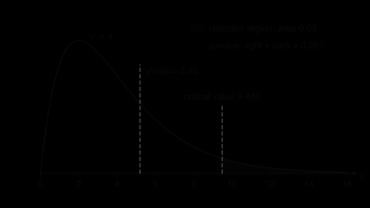
Chi-squared distribution curve with 4 degrees of freedom. The area to the right of the critical value 9.488 is shaded dark: the rejection region, area 0.05. The area to the right of the statistic 5.20 is shaded light plus dark: the p-value, 0.267. — With 4 degrees of freedom at the 5% level, the statistic 5.20 lies left of the critical value 9.488, and the area beyond it, the p-value 0.267, is larger than 0.05: both comparisons lead to the same decision.

The chi-squared curve with 4 degrees of freedom shows both methods at once: the statistic 5.20 lies outside the rejection region, and the p-value of 0.267 is larger than 0.05, so $\mathrm{H}_0$ is not rejected.

Compare	Reject $\mathrm{H}_0$ when	Do not reject $\mathrm{H}_0$ when
p-value with significance level	p-value < significance level	p-value ≥ significance level
$\chi^2_{calc}$ with critical value	$\chi^2_{calc}$ > critical value	$\chi^2_{calc}$ ≤ critical value

Steps of every test

Every hypothesis test, whatever its type, is set out in the same five steps. The flowchart summarises them.

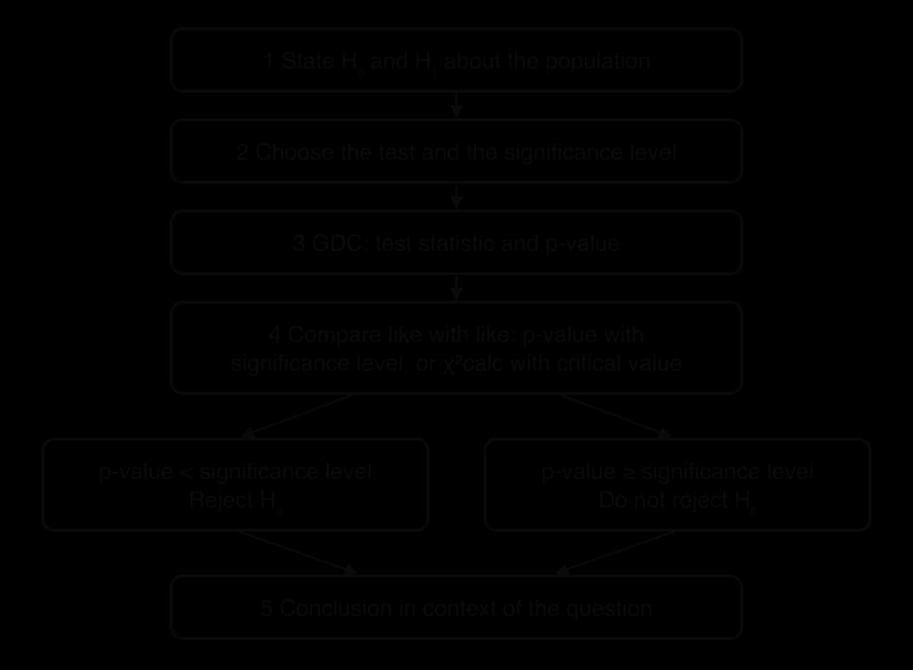
Flowchart of a hypothesis test: 1 state H0 and H1 about the population; 2 choose the test and significance level; 3 GDC gives statistic and p-value; 4 compare like with like; reject H0 if p-value < significance level, otherwise do not reject; 5 conclude in context. — Every test has the same structure; only step 3, the calculation, changes from one test to another.

State $\mathrm{H}_0$ and $\mathrm{H}_1$ about the population.
Choose the test and the significance level (often given).
Calculate the test statistic and the p-value with the GDC.
Compare the p-value with the significance level (or the statistic with the critical value).
Write the decision and a conclusion in the context of the question.

The final step matters as much as the calculation. "Reject $\mathrm{H}_0$ " on its own says nothing about rabbits, dice or fertilisers; the conclusion must translate the decision back into the situation, for example "there is evidence, at the 5% level, that the mean height of plants grown with fertiliser A differs from the mean height with fertiliser B".

In three separate tests the p-values are 0.0372, 0.0085 and 0.124. Determine the decision for each test at the 1%, 5% and 10% significance levels.

Show the solution

Reject $\mathrm{H}_0$ whenever the p-value is less than the significance level.

p-value	1% (0.01)	5% (0.05)	10% (0.10)
0.0372	do not reject	reject	reject
0.0085	reject	reject	reject
0.124	do not reject	do not reject	do not reject

The p-value 0.0372 shows how the level changes the decision: it is significant at the 5% and 10% levels but not at the 1% level. This is why the significance level is fixed before the data are seen.

Observed and expected frequencies

The two chi-squared tests deal with counts: how many people, seeds or rolls fall into each category. The data are categorical, or numerical data grouped into classes. The counts recorded in the sample are compared with the counts that $\mathrm{H}_0$ predicts.

The predicted counts come from the probabilities in $\mathrm{H}_0$ , using the idea of an expected number of occurrences from subtopic 4.5: if an outcome has probability $p$ on each of $n$ independent trials, it is expected to occur $np$ times.

Expected frequencies do not need to be whole numbers. An expected frequency of 21.8 is an average over many possible samples, in the same way that a family can have an average of 1.6 children. Rounding them to whole numbers before calculating the statistic introduces avoidable error.

Measuring the discrepancy: the chi-squared statistic

To judge whether observed and expected frequencies are far apart, the differences $f_o - f_e$ in every category are combined into one number. Three features of the formula each have a reason.

Squaring. The differences always add to zero (the totals of $f_o$ and $f_e$ are equal), so they must be squared to stop positive and negative differences cancelling.
Dividing by $f_e$ . A difference of 10 is large when 20 are expected and trivial when 2,000 are expected. Dividing by the expected frequency measures each squared difference relative to the size of the category.
Adding. Every category contributes, so a large departure anywhere increases the total.

\chi^2_{calc} = \sum \frac{\left(f_o - f_e\right)^2}{f_e}

The result $\chi^2_{calc}$ is zero only when every observed frequency equals its expected frequency, and grows as the data move away from $\mathrm{H}_0$ . Only large values count as evidence against $\mathrm{H}_0$ , which is why chi-squared tests are upper-tail tests. The GDC carries out exactly this calculation, so a hand calculation on a small table is a good check on the GDC entries.

The chi-squared distribution and degrees of freedom

If $\mathrm{H}_0$ is true and the expected frequencies are not too small, the values of $\chi^2_{calc}$ from repeated samples follow a known probability distribution. Its shape depends on how many of the frequencies are free to vary.

The totals in a table act as constraints. In a goodness of fit test with 6 categories and a total of 90, once five frequencies are known, the sixth is fixed: it must make the total 90. Only five frequencies are free to vary.

The graph of the chi-squared distribution for three values of $\nu$ shows how the curve spreads to the right as the number of degrees of freedom increases. The mean of the distribution equals $\nu$ , so a statistic of 6 is unremarkable with 8 degrees of freedom but quite large with 2.

ν = 2
ν = 4
ν = 8

As the degrees of freedom increase, the chi-squared curve moves to the right and spreads out, so larger statistics are needed before they count as unusual.

The critical values that cut off an upper tail of 10%, 5% or 1% come from this distribution. They are given in questions when needed, but the table shows typical values and how they grow with $\nu$ .

$\nu$	10%	5%	1%
2	4.605	5.991	9.210
3	6.251	7.815	11.345
4	7.779	9.488	13.277
5	9.236	11.070	15.086
6	10.645	12.592	16.812
8	13.362	15.507	20.090

Upper-tail critical values of the chi-squared distribution, calculated with technology.

The chi-squared goodness of fit test

A goodness of fit test checks whether a set of observed frequencies is consistent with a stated probability distribution: equal probabilities (a fair die or spinner), probabilities in a given ratio (a genetic cross), given percentages (a company's claim), or probabilities from a named distribution such as the normal distribution with given mean and standard deviation.

The method follows the general steps, with the expected frequencies coming from the stated distribution.

$\mathrm{H}_0$ : the data fit the stated distribution (naming it). $\mathrm{H}_1$ : the data do not fit it.
Find each expected frequency: total frequency × probability of the category under $\mathrm{H}_0$ .
Degrees of freedom: $\nu = n - 1$ , where $n$ is the number of categories (the only constraint is that the expected frequencies add up to the same total as the observed ones).
Find $\chi^2_{calc}$ and the p-value with the GDC.
Compare and conclude in context.

The test is reliable only when every expected frequency is greater than 5. With very small expected frequencies, dividing by $f_e$ makes single chance observations produce large contributions, and the chi-squared distribution no longer describes the statistic well. When some expected frequencies are 5 or less, neighbouring categories are combined, a method HL students meet in subtopic 4.12.

By hand and on the GDC: testing a die

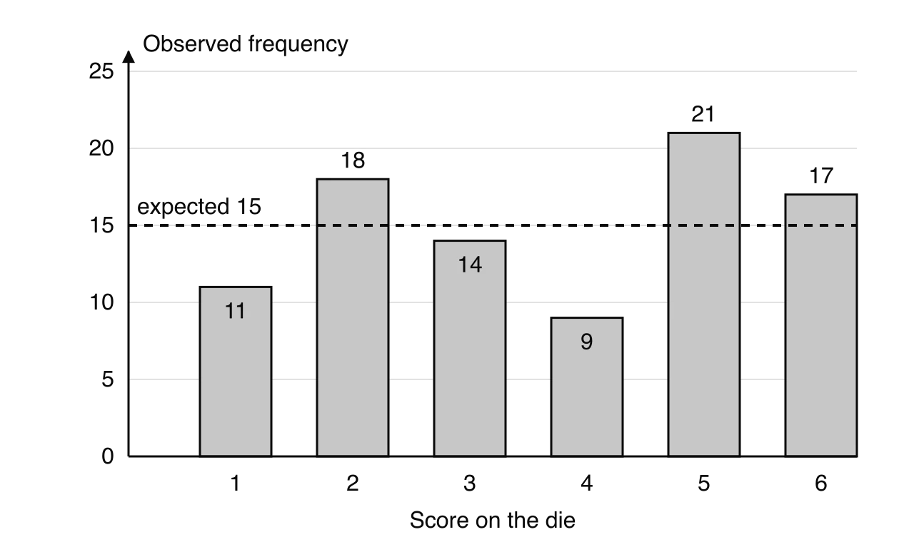
A die is rolled 90 times and the scores 1 to 6 appear 11, 18, 14, 9, 21 and 17 times. If the die is fair, each score has probability $\frac{1}{6}$ and expected frequency 15. The bar chart of the observed frequencies against the expected value shows the size of the differences that the test must judge.

Bar chart of 90 rolls of a die: observed frequencies 11, 18, 14, 9, 21 and 17 for scores 1 to 6, with a dashed horizontal line at the expected frequency 15 for every score. — Observed frequencies scatter around the expected 15; the test decides whether differences of up to 6 are larger than chance would usually produce in 90 rolls.

Score	1	2	3	4	5	6
Frequency	11	18	14	9	21	17

Scores from 90 rolls of a die (hypothetical data).

A die is rolled 90 times, with the frequencies of the scores shown in the table of 90 rolls. A chi-squared goodness of fit test at the 5% significance level is used to test whether the die is fair.

(a) State the hypotheses. (b) Calculate $\chi^2_{calc}$ by hand. (c) Write down the degrees of freedom. (d) Find the p-value and state the conclusion.

Show the solution

(a) $\mathrm{H}_0$ : the die is fair (each score has probability $\frac{1}{6}$ ). $\mathrm{H}_1$ : the die is not fair.

(b) Each expected frequency is $90 \times \frac{1}{6} = 15$ .

Score	$f_o$	$f_e$	$f_o - f_e$	$\frac{(f_o - f_e)^2}{f_e}$
1	11	15	−4	1.0667
2	18	15	3	0.6
3	14	15	−1	0.0667
4	9	15	−6	2.4
5	21	15	6	2.4
6	17	15	2	0.2667

\chi^2_{calc} = 1.0667 + 0.6 + 0.0667 + 2.4 + 2.4 + 0.2667 = 6.8

(d) Using the GDC's chi-squared goodness of fit test with the observed frequencies in one list, the expected frequencies in another and $\nu = 5$ :

\chi^2_{calc} = 6.80, \quad \text{p-value} = 0.236

Since $0.236 > 0.05$ , do not reject $\mathrm{H}_0$ . There is insufficient evidence at the 5% level to conclude that the die is unfair. The differences from 15 are of the size that chance often produces in 90 rolls of a fair die.

GDC procedure for goodness of fit

The GDC needs the observed and expected frequencies in two lists, in the same order.

Enter the observed frequencies in one list (for example L1) and the expected frequencies in another (L2).
Run the goodness of fit test: on a TI-84 Plus CE, STAT → TESTS → χ²GOF-Test; on a Casio fx-CG50, MENU → Statistics → TEST → CHI → GOF.
Enter the observed list, the expected list and the degrees of freedom $n - 1$ .
Read off $\chi^2$ and the p-value.

On paper, write the hypotheses, the expected frequencies, the degrees of freedom, $\chi^2_{calc}$ and the p-value, then the comparison and conclusion. Calculator syntax such as "χ²GOF-Test(L1, L2, 5)" is not mathematical notation, so it is no substitute for these values.

Given ratios and percentages

When $\mathrm{H}_0$ gives probabilities in a ratio, each ratio part is converted to a fraction of the total. A ratio of $9 : 3 : 3 : 1$ has 16 parts, so the probabilities are $\frac{9}{16}$ , $\frac{3}{16}$ , $\frac{3}{16}$ and $\frac{1}{16}$ . Given percentages are used directly as probabilities.

A manufacturer states that the sweets in its mixed bags are 30% red, 25% yellow, 20% green, 15% orange and 10% purple. A random sample of 200 sweets contains 52 red, 61 yellow, 37 green, 31 orange and 19 purple. A goodness of fit test is carried out at the 5% significance level; the critical value is 9.488.

(a) Find the expected frequencies. (b) Write down the number of degrees of freedom. (c) Find $\chi^2_{calc}$ . (d) State the conclusion, giving a reason.

Show the solution

$\mathrm{H}_0$ : the colours occur in the proportions the manufacturer states. $\mathrm{H}_1$ : the colours do not occur in these proportions.

(a) Expected frequency = $200 \times$ percentage.

Colour	Red	Yellow	Green	Orange	Purple
$f_o$	52	61	37	31	19
$f_e$	60	50	40	30	20

(b) 5 categories, so $\nu = 5 - 1 = 4$ .

(d) Since $3.80 < 9.488$ , do not reject $\mathrm{H}_0$ . There is insufficient evidence at the 5% level that the colours differ from the manufacturer's stated proportions.

The critical-value comparison in that example reaches the same decision as the p-value: $0.434 > 0.05$ .

Testing a genetic ratio: Mendel's peas

In his 1866 paper on plant hybridisation, Gregor Mendel crossed pea plants and counted the seeds in the second generation by two features: shape (round or wrinkled) and colour (yellow or green). His theory of inheritance predicts the four types in the ratio $9 : 3 : 3 : 1$ . His counts for 556 seeds were 315 round and yellow, 108 round and green, 101 wrinkled and yellow, and 32 wrinkled and green.

Seed type	Round, yellow	Round, green	Wrinkled, yellow	Wrinkled, green
Observed $f_o$	315	108	101	32
Probability under $\mathrm{H}_0$	$\frac{9}{16}$	$\frac{3}{16}$	$\frac{3}{16}$	$\frac{1}{16}$
Expected $f_e$	312.75	104.25	104.25	34.75

Source: G. Mendel, "Experiments in plant hybridization" (1866), English translation published by MendelWeb.

Use Mendel's counts to perform a chi-squared goodness of fit test, at the 5% significance level, of the hypothesis that the four seed types occur in the ratio $9 : 3 : 3 : 1$ . Interpret the result.

Show the solution

$\mathrm{H}_0$ : the seed types occur in the ratio $9 : 3 : 3 : 1$ . $\mathrm{H}_1$ : the seed types do not occur in this ratio.

Expected frequencies: $556 \times \frac{9}{16} = 312.75$ , $556 \times \frac{3}{16} = 104.25$ (twice) and $556 \times \frac{1}{16} = 34.75$ . All are greater than 5.

Degrees of freedom: $\nu = 4 - 1 = 3$ .

From the GDC: $\chi^2_{calc} = 0.470$ , p-value $= 0.925$ .

Since $0.925 > 0.05$ , do not reject $\mathrm{H}_0$ . The data are very consistent with the $9 : 3 : 3 : 1$ ratio that Mendel's theory predicts.

The p-value of 0.925 means that a random sample from a true $9 : 3 : 3 : 1$ population would differ from the expected counts more than Mendel's did about 92.5% of the time. Mendel's fit is unusually close.

Mendel's results as a whole have been examined in the same way. In 1936 the statistician R. A. Fisher applied the chi-squared test to Mendel's experiments as a whole and argued that the results were too close to the predicted ratios to be plausible, suggesting that the data had been adjusted, consciously or not. Later researchers have disputed parts of Fisher's analysis. The lesson for hypothesis testing is that a p-value very close to 1 is not "proof" of a model. Across many experiments, p-values from a true model are spread out between 0 and 1, so a long run of near-perfect fits is itself a pattern that needs explaining.

Goodness of fit to a normal model

A goodness of fit test can check whether continuous data follow a normal distribution with a given mean and standard deviation. The data are grouped into classes, and the expected frequency of each class is the total multiplied by the normal probability of that class, found with the GDC's normal cumulative distribution function as in subtopic 4.9. The first and last classes are open-ended so that the probabilities add up to 1.

Mass $m$ (g)	$m < 140$	$140 \le m < 150$	$150 \le m < 160$	$160 \le m < 170$	$m \ge 170$
Frequency	72	125	160	100	43

Masses of a random sample of 500 apples (hypothetical data).

The masses of apples from an orchard are thought to follow $\mathrm{N}(152, 12^2)$ , in grams. A random sample of 500 apples gives the grouped frequencies in the table.

(a) Find the expected frequency of apples with $m < 140$ , correct to 4 significant figures. [2]

(b) Find the remaining expected frequencies. [2]

(d) Find the p-value and state the conclusion at the 5% significance level. [4]

Show the solution

(a) Let $M \sim \mathrm{N}(152, 12^2)$ . Then $\mathrm{P}(M < 140) = 0.158655\ldots$ (M1)

Expected frequency $= 500 \times 0.158655\ldots = 79.33$ A1

(b) Each probability is found from the normal distribution and multiplied by 500.

Class	$m < 140$	$140$ – $150$	$150$ – $160$	$160$ – $170$	$m \ge 170$
Probability	0.15866	0.27516	0.31369	0.18569	0.06681
$f_e$	79.33	137.6	156.8	92.84	33.40

A1A1

$\mathrm{H}_1$ : the masses cannot be modelled by $\mathrm{N}(152, 12^2)$ . A1

(d) Five categories, so $\nu = 4$ . (A1)

From the GDC, $\chi^2_{calc} = 5.20$ and p-value $= 0.267$ . A1

$0.267 > 0.05$ R1

There is insufficient evidence to reject $\mathrm{H}_0$ : the masses are consistent with the model $\mathrm{N}(152, 12^2)$ . A1

The largest contribution, 2.76, comes from the heaviest class (43 observed against 33.4 expected), a hint that the model may slightly underestimate the number of heavy apples, but not by enough to be significant.

CrashCourse, “Chi-Square Tests: Crash Course Statistics #29”: follow how observed and expected counts are compared in both a goodness of fit test and a test for independence.

Contingency tables and the chi-squared test for independence

Many questions ask whether two categorical variables are connected: whether choice of transport depends on year group, whether survival depended on class of ticket, whether preferred holiday depends on age. Data on two categorical variables are displayed in a table with one variable along the rows and the other along the columns, extending the two-way tables of subtopic 4.6.

The test asks whether the pattern in the table could have arisen by chance if the two variables were independent in the population.

Expected frequencies under independence

The expected frequencies come straight from the definition of independent events, $\mathrm{P}(A \cap B) = \mathrm{P}(A)\,\mathrm{P}(B)$ . In a survey of 200 students, suppose 100 are in Grade 11 and 56 walk to school. If year group and transport are independent, the probability that a randomly chosen student is in Grade 11 and walks is

\mathrm{P}(\text{Grade 11} \cap \text{walk}) = \frac{100}{200} \times \frac{56}{200}

so the expected number of Grade 11 walkers among the 200 is

f_e = 200 \times \frac{100}{200} \times \frac{56}{200} = \frac{100 \times 56}{200} = 28

One factor of 200 cancels, giving the rule used for every cell.

f_e = \frac{\text{row total} \times \text{column total}}{\text{grand total}}

The rule keeps the row and column totals of the expected table equal to those of the observed table, which is why the totals act as constraints.

Degrees of freedom for a contingency table

The degrees of freedom count the cells that can be filled freely once all the row and column totals are fixed. In a table with 2 rows and 3 columns, once the first two cells of the first row are chosen, the third is fixed by the row total; the whole second row is then fixed by the column totals. Only 2 cells are free. In general, the last cell in each row and the last row are determined by the totals.

\nu = (r - 1)(c - 1)

where $r$ is the number of rows and $c$ the number of columns, not counting the totals. A table with 3 rows and 4 columns has $\nu = 2 \times 3 = 6$ .

	Walk	Bus	Car	Total
Grade 11	34	41	25	100
Grade 12	22	30	48	100
Total	56	71	73	200

Method of travel to school by year group (hypothetical data).

A random sample of 100 Grade 11 and 100 Grade 12 students at a school were asked how they usually travel to school, with the results shown in the table of travel methods.

(a) Calculate the expected frequencies. (b) Calculate $\chi^2_{calc}$ by hand. (c) Perform a chi-squared test for independence at the 1% significance level.

Show the solution

(a) Using $f_e = \frac{\text{row total} \times \text{column total}}{\text{grand total}}$ , for example $\frac{100 \times 71}{200} = 35.5$ for Grade 11 by bus. Both rows have total 100, so both rows have the same expected frequencies.

	Walk	Bus	Car
Grade 11	28	35.5	36.5
Grade 12	28	35.5	36.5

(b) The contributions $\frac{(f_o - f_e)^2}{f_e}$ are

	Walk	Bus	Car
Grade 11	$\frac{6^2}{28} = 1.286$	$\frac{5.5^2}{35.5} = 0.852$	$\frac{11.5^2}{36.5} = 3.623$
Grade 12	$\frac{6^2}{28} = 1.286$	$\frac{5.5^2}{35.5} = 0.852$	$\frac{11.5^2}{36.5} = 3.623$

\chi^2_{calc} = 2(1.286 + 0.852 + 3.623) = 11.5 \text{ (3 s.f.)}

(c) $\mathrm{H}_0$ : method of travel and year group are independent. $\mathrm{H}_1$ : method of travel and year group are not independent.

$\nu = (2 - 1)(3 - 1) = 2$ .

From the GDC, $\chi^2_{calc} = 11.5$ , p-value $= 0.00315$ .

Since $0.00315 < 0.01$ , reject $\mathrm{H}_0$ . There is evidence at the 1% level that method of travel to school is not independent of year group. The largest contributions come from the car column: more Grade 12 students and fewer Grade 11 students travel by car than independence predicts, which fits older students being more likely to drive or be driven.

GDC procedure for independence

The GDC takes the observed table as a matrix and produces the statistic, the p-value and the degrees of freedom, and stores the expected frequencies.

Enter the observed frequencies, without the totals, as a matrix with $r$ rows and $c$ columns: on a TI-84 Plus CE, 2nd x⁻¹ (MATRIX) → EDIT → [A]; on a Casio fx-CG50, the matrix is entered from the test screen's Observed field (Mat A).
Run the test: TI-84 Plus CE STAT → TESTS → χ²-Test with Observed [A] and Expected [B]; Casio fx-CG50 MENU → Statistics → TEST → CHI → 2WAY.
Read off $\chi^2$ , the p-value and df. The expected frequencies are stored in matrix [B] (TI) or can be viewed from the result screen (Casio), which helps with questions asking for one expected value.

Write down the hypotheses, $\nu$ , $\chi^2_{calc}$ , the p-value, the comparison and the conclusion. When an expected frequency is asked for, show the substitution into the formula as well as the value.

Interpreting the result

A significant result says that the two variables are associated in the population: the proportions in the categories of one variable differ between the categories of the other. Comparing each observed frequency with its expected frequency, or looking at the largest contributions to $\chi^2_{calc}$ , shows where the association lies. The test does not show that one variable causes the other, and it does not measure how strong the association is; a very large sample can make a weak association significant.

Case study: survival on the Titanic

When the Titanic sank in April 1912, the British Board of Trade inquiry recorded how many people in each class were saved and lost. The 2,201 people on board are classified by two categorical variables: class (first, second, third, crew) and outcome (saved, lost).

	Saved	Lost	Total
First class	202	123	325
Second class	118	167	285
Third class	178	528	706
Crew	212	673	885
Total	710	1,491	2,201

Source: British Board of Trade inquiry report (Mersey, 1912), as tabulated in the Wikipedia article "Sinking of the Titanic", retrieved 2026.

Of the 2,201 people on board, $\frac{710}{2201} \approx 32.3\%$ survived. If survival had been independent of class, about 32.3% of every class would have been saved. The expected frequencies follow from the row-total × column-total rule; for first class saved, $\frac{325 \times 710}{2201} = 104.8$ .

	Saved ( $f_o$ )	Saved ( $f_e$ )	Lost ( $f_o$ )	Lost ( $f_e$ )
First class	202	104.8	123	220.2
Second class	118	91.9	167	193.1
Third class	178	227.7	528	478.3
Crew	212	285.5	673	599.5

With $\mathrm{H}_0$ : class and survival are independent, the table has 4 rows and 2 columns, so $\nu = (4 - 1)(2 - 1) = 3$ . The GDC gives $\chi^2_{calc} = 187.8$ and a p-value of about $1.8 \times 10^{-40}$ , far below any usual significance level, so $\mathrm{H}_0$ is rejected: survival was not independent of class. The first-class "saved" cell alone contributes 90.0 to the statistic, with nearly twice as many first-class survivors as independence predicts. The survival rates were about 62% in first class, 41% in second, 25% in third and 24% among the crew.

The result needs careful interpretation. The 2,201 people are the whole population of the voyage rather than a random sample, so the test is best read as asking whether differences this large could plausibly be the result of chance alone; a p-value this small rules that out. The test also says nothing about the reasons. Class was tied to other factors: the crew were almost all men, at a time when women and children were put into the lifeboats first, and third-class cabins were further from the boat deck. An association between class and survival is not, by itself, evidence that the ticket class caused the difference.

A full test for independence

A typical question on a test for independence gives a contingency table with its totals and asks for each part of the test in turn.

Age group	Beach	City	Adventure	Total
18–30	38	29	13	80
31–50	27	35	18	80
Over 50	15	16	29	60
Total	80	80	60	220

Preferred type of holiday by age group (hypothetical data).

A travel company surveys a random sample of 220 customers about their preferred type of holiday. The results, by age group, are shown in the table.

A chi-squared test for independence is carried out at the 1% significance level. The critical value is 13.277.

(a) State the null hypothesis. [1]

(b) Show that the expected frequency of customers over 50 who prefer an adventure holiday is 16.4, correct to 3 significant figures. [2]

(d) Write down the value of $\chi^2_{calc}$ . [2]

(e) State the conclusion of the test, giving a reason. [2]

Show the solution

(a) $\mathrm{H}_0$ : preferred type of holiday and age group are independent. A1

(b) $\frac{60 \times 60}{220}$ M1

$= 16.3636\ldots = 16.4$ A1

Both the unrounded and the rounded value are shown, as a "show that" requires.

(d) From the GDC with the 3 × 3 matrix of observed frequencies: $\chi^2_{calc} = 21.8$ (21.7517…) A2

(e) $21.8 > 13.277$ R1

Reject $\mathrm{H}_0$ : there is evidence at the 1% level that preferred type of holiday is not independent of age group. A1

(The p-value is 0.000225, which also gives $0.000225 < 0.01$ .) The largest contribution comes from customers over 50 choosing adventure holidays: 29 observed against 16.4 expected.

The t-test

The chi-squared tests compare counts. Many investigations instead compare a numerical variable between two groups: the heights of plants given two fertilisers, the reaction times of drivers with and without a phone, the lifetimes of two brands of battery. The natural question is whether the two population means differ.

The test used for this question was devised by William Sealy Gosset, a chemist at the Guinness brewery in Dublin who needed to judge the quality of ingredients from very small samples. Guinness did not allow its staff to publish under their own names, so he published the method in the journal Biometrika in 1908 under the pen name "Student", and it is still called Student's t-test.

The idea behind the t-statistic

Two sample means will almost always differ, even if the population means are equal. Whether a difference is convincing depends on how large it is compared with the variation inside the samples and on how big the samples are. A difference of 2 cm in mean height is strong evidence if every plant in each group is within a few millimetres of its group's mean, and weak evidence if heights vary by 10 cm within each group.

The graph shows normal curves centred at the two sample means of an example comparing two fertilisers, each with the common spread of the data. The curves overlap a great deal; the t-test judges whether the gap between the centres is still larger than chance would usually give.

fertiliser A
fertiliser B

The sample means differ by 1.86 cm while each group spreads over several centimetres; the t-test weighs that gap against the spread and the sample sizes.

The GDC calculates a t-statistic that has exactly this structure: the difference in sample means divided by a measure of how much that difference would vary from sample to sample.

How the GDC calculates the pooled t-statistic (optional)

For samples of sizes $n_1$ and $n_2$ with means $\bar{x}_1$ , $\bar{x}_2$ and sample standard deviations $s_1$ , $s_2$ (calculated with divisor $n - 1$ ), the pooled standard deviation combines the two samples' variation:

s_p = \sqrt{\frac{(n_1 - 1)s_1^2 + (n_2 - 1)s_2^2}{n_1 + n_2 - 2}}

t = \frac{\bar{x}_1 - \bar{x}_2}{s_p\sqrt{\dfrac{1}{n_1} + \dfrac{1}{n_2}}}

The statistic follows a t-distribution with $n_1 + n_2 - 2$ degrees of freedom when $\mathrm{H}_0$ is true. For the fertiliser data, $s_p = 1.3105$ and $t = \frac{1.8625}{1.3105 \times 0.5} = 2.84$ . In practice the GDC does this calculation.

Assumptions of the pooled t-test

The p-value from a t-test means what it should only when these conditions hold.

The two samples are independent random samples (unpaired: different individuals in each group).
Each population is normally distributed. With small samples this matters; a box-and-whisker diagram or histogram of each sample that looks roughly symmetric with no outliers supports the assumption.
The two populations have equal variances, so the samples' variation can be combined ("pooled") into one estimate. Sample standard deviations of similar size make this assumption reasonable.
The population variances are unknown and estimated from the samples.

If the data are strongly skewed or have outliers, the t-test is not appropriate. Psychology and biology often use the Mann–Whitney U test in that situation, which compares ranks instead of means.

GDC procedure for the t-test

Enter the two samples in two lists (L1 and L2).
Run the two-sample t-test: on a TI-84 Plus CE, STAT → TESTS → 2-SampTTest; on a Casio fx-CG50, MENU → Statistics → TEST → t → 2-S.
Choose data input (lists), select the alternative hypothesis ( $\ne$ , $<$ or $>$ , with $\mu_1$ for the first list), and set Pooled: Yes (Casio: Pooled On).
Read off $t$ and the p-value.

On paper, define $\mu_1$ and $\mu_2$ , state the hypotheses, name the test ("pooled two-sample t-test"), and write the p-value, the comparison and the conclusion about the population means.

Fertiliser A	24.1	26.3	22.8	25.5	27.0	23.9	25.2	26.6
Fertiliser B	22.4	23.8	21.9	24.6	23.1	25.0	22.2	23.5

Heights of tomato plants, in cm, after six weeks (hypothetical data).

A gardener grows 8 tomato plants with fertiliser A and 8 with fertiliser B, and measures their heights after six weeks; the table of heights gives the results.

The heights are assumed to be normally distributed with equal variances. Perform a t-test at the 5% significance level to test whether the mean heights differ.

Show the solution

Let $\mu_A$ and $\mu_B$ be the population mean heights of plants grown with fertilisers A and B.

$\mathrm{H}_0$ : $\mu_A = \mu_B$ . $\mathrm{H}_1$ : $\mu_A \ne \mu_B$ . The question asks whether the means differ, with no direction, so the test is two-tailed.

Using the GDC's pooled two-sample t-test with the data in two lists and alternative $\mu_1 \ne \mu_2$ :

t = 2.84, \quad \text{p-value} = 0.0130

Since $0.0130 < 0.05$ , reject $\mathrm{H}_0$ . There is evidence at the 5% level that the mean height of tomato plants grown with fertiliser A differs from the mean height with fertiliser B. The sample means (25.2 cm and 23.3 cm) suggest that fertiliser A gives taller plants on average.

The conclusion refers to the mean heights of all plants that could be grown with each fertiliser, rather than to the 16 plants measured. It is also limited to the conditions of the experiment: one variety, six weeks, one garden.

One-tailed and two-tailed tests

The alternative hypothesis of a t-test can take two forms, and the choice depends on the question asked before the data are collected.

A two-tailed test is used for claims such as "the means differ" or "the new method changes the mean". Evidence against $\mathrm{H}_0$ comes from a large difference in either direction, so the p-value counts extreme results at both ends of the distribution.

A one-tailed test is used for claims with a direction: "heavier", "faster", "improves", "reduces", "less than". Only differences in the stated direction count as evidence, so the p-value counts only one end of the distribution. When the sample difference is in the stated direction, the one-tailed p-value is half the two-tailed p-value, because the distribution of $t$ is symmetric.

Claim in the question	$\mathrm{H}_1$	Type
"The mean weights are different"	$\mu_1 \ne \mu_2$	two-tailed
"Group 1 is heavier on average"	$\mu_1 > \mu_2$	one-tailed
"Group 1 has a lower mean"	$\mu_1 < \mu_2$	one-tailed

The direction is fixed by the claim before the data are examined. Choosing $\mu_1 > \mu_2$ after noticing that $\bar{x}_1 > \bar{x}_2$ halves the p-value unfairly and makes a significant result more likely than the significance level allows.

A teacher claims that a new revision method raises mean test scores. Ten students using the new method and ten different students using the old method score as follows.

New method: 68, 74, 71, 80, 77, 65, 73, 79, 70, 76

Old method: 66, 71, 64, 73, 75, 61, 69, 72, 68, 73

Scores are assumed normal with equal variances.

(a) Perform a suitable t-test at the 5% level to test the teacher's claim. (b) A colleague tests whether the mean scores differ, at the same level. Find the colleague's p-value and explain why the two conclusions differ.

Show the solution

(a) Let $\mu_N$ and $\mu_O$ be the population mean scores for the new and old methods.

$\mathrm{H}_0$ : $\mu_N = \mu_O$ . $\mathrm{H}_1$ : $\mu_N > \mu_O$ (the claim says "raises", so one-tailed).

Pooled two-sample t-test, alternative $\mu_1 > \mu_2$ : $t = 1.97$ , p-value $= 0.0325$ .

Since $0.0325 < 0.05$ , reject $\mathrm{H}_0$ . There is evidence at the 5% level that the new method raises the mean test score, which supports the teacher's claim.

(b) With $\mathrm{H}_1$ : $\mu_N \ne \mu_O$ , the GDC gives p-value $= 0.0650$ (twice 0.0325).

Since $0.0650 > 0.05$ , the colleague does not reject $\mathrm{H}_0$ .

The one-tailed test puts all 5% of the rejection probability in the direction of the claim, so a smaller difference in that direction is enough. The two-tailed test splits it between both directions, so the same difference is not extreme enough. Both tests are correct for their own question, which is why the hypotheses must be fixed before the data are examined.

The chi-squared tests have non-directional hypotheses ("independent" or "not independent"; "fits" or "does not fit"), yet the calculation uses only the upper tail of the chi-squared distribution. Departures from $\mathrm{H}_0$ in any direction make $\chi^2_{calc}$ larger, because the differences are squared, so all the evidence against $\mathrm{H}_0$ lies in the upper tail and the two ideas are consistent.

Choosing and reporting a test

Choosing the right test depends on the type of data and on the question.

Situation	Data	Test	Degrees of freedom
Are two categorical variables connected?	Counts in a contingency table	Chi-squared test for independence	$(r - 1)(c - 1)$
Do counts follow a stated distribution?	Counts in $n$ categories	Chi-squared goodness of fit test	$n - 1$
Do two population means differ?	Numerical values in two independent samples	Pooled two-sample t-test	handled by the GDC

A complete test, set out in full, contains:

hypotheses about the population, in words or in symbols with the symbols defined;
the test used (and degrees of freedom for a chi-squared test);
the test statistic and/or p-value from the GDC (with expected frequencies where relevant);
a numerical comparison with the significance level or critical value;
the decision and a conclusion in context.

Statistical significance is also different from practical importance. A test on 10,000 people might find that one teaching method gives a mean score 0.3 points higher than another with a p-value of 0.001; the difference is statistically significant but too small to matter in practice. Results are best reported with the sample means or proportions, so that a reader can judge the size of the effect as well as its significance.

Exam focus

Hypothesis testing is one of the most frequently examined SL subtopics, on Paper 1 as a 4–8 mark question and on Paper 2 as part of a longer question, often after earlier parts on probabilities from the same table or on the normal distribution. Questions use state (the hypotheses, the conclusion), write down (degrees of freedom, $\chi^2_{calc}$ , the p-value from the GDC), find or calculate (an expected frequency, the p-value), show that (an expected frequency rounds to a given value) and perform (the whole test: hypotheses, p-value, comparison and conclusion). Critical values are given when needed. Recurring shapes are: a contingency table with an expected frequency, df, the statistic and a conclusion; a goodness of fit test for a die, equal daily sales or a normal model with expected frequencies from normal probabilities; and a pooled t-test with raw data and a stated claim.

A company tests two brands of rechargeable battery. It claims that brand X batteries last longer, on average, than brand Y batteries. A random sample of batteries of each brand is tested, and the lifetimes, in hours, are recorded.

Brand X: 41.2, 44.5, 39.8, 46.1, 43.0, 42.7, 45.3

Brand Y: 38.9, 41.5, 40.2, 37.6, 42.8, 39.4, 40.7, 41.1

A t-test is carried out at the 5% significance level to test the company's claim.

(a) State the null and alternative hypotheses. [2]

(b) Find the p-value for this test. [2]

(d) State one assumption about the lifetimes that is needed for the test to be valid. [1]

(e) The company repeats its test at the 1% significance level. A technician uses the same data to test whether the mean lifetimes are different, also at the 1% level.

(i) Write down the technician's p-value. [1]

(ii) Explain why the two tests at the 1% level reach different conclusions. [2]

Show the markscheme

(a) Let $\mu_X$ and $\mu_Y$ be the population mean lifetimes of brand X and brand Y batteries.

$\mathrm{H}_0$ : $\mu_X = \mu_Y$ A1

$\mathrm{H}_1$ : $\mu_X > \mu_Y$ A1

Accept equivalent statements in words that refer to the population mean (or the mean lifetime of all batteries of each brand). Do not accept statements about the sample means.

(b) Pooled two-sample t-test: p-value $= 0.00572$ (0.0057210…) A2

Award A1 for 0.00765 (unpooled).

Reject $\mathrm{H}_0$ : there is evidence at the 5% level that brand X batteries last longer on average than brand Y batteries; the company's claim is supported. A1

Do not award R0A1.

(d) The lifetimes of each brand are normally distributed (or: the two populations have equal variances; or: the samples are independent and random). A1

(e)(i) p-value $= 0.0114$ (0.011442…) A1

(ii) The two-tailed p-value is double the one-tailed p-value ( $0.0114 = 2 \times 0.00572$ ) R1

At the 1% level, $0.00572 < 0.01$ so the company's one-tailed test rejects $\mathrm{H}_0$ , while $0.0114 > 0.01$ so the technician's two-tailed test does not reject $\mathrm{H}_0$ . R1

Total [10]

The wording of hypotheses carries marks on its own and is where marks are most often lost.

A conclusion is marked in two parts: a reason mark for the numerical comparison and an accuracy mark for the decision. The decision mark is not awarded without the comparison, so writing "reject $\mathrm{H}_0$ " alone scores nothing.

Practice questions

A shop records each customer's method of payment (cash, card or phone) and whether they shop on a weekday or at the weekend. State the null and alternative hypotheses for a chi-squared test for independence. [2]
In a contingency table with grand total 150, a cell is in a row with total 45 and a column with total 60. Calculate the expected frequency for that cell. [2]
Write down the number of degrees of freedom for (a) a test for independence using a table with 4 rows and 3 columns; (b) a goodness of fit test with 7 categories. [2]
A call centre receives 220 calls in one week: 48 on Monday, 39 on Tuesday, 35 on Wednesday, 42 on Thursday and 56 on Friday. Test, at the 5% level, whether calls are equally likely on each weekday. The critical value is 9.488. State the hypotheses, write down $\chi^2_{calc}$ and state the conclusion with a reason. [5]
Students at two campuses choose one club.

	Sport	Music	Drama
Campus A	18	27	15
Campus B	32	21	7

Perform a chi-squared test for independence at the 1% level. State whether the conclusion would change at the 5% level. [6]

Leaf lengths, in cm, at two sites are: Site 1: 12.4, 13.1, 11.8, 12.9, 13.5, 12.2; Site 2: 11.6, 12.0, 12.7, 11.3, 12.1, 11.9. Assuming normal populations with equal variances, perform a t-test at the 5% level of whether the population mean lengths differ. [6]
A genetic model predicts offspring of three types in the ratio $1 : 2 : 1$ . Of 150 offspring, 38, 61 and 51 are of the three types. Find the expected frequencies, the p-value and the conclusion at the 5% level. [6]
A test at the 1% significance level gives a p-value of 0.03. State the conclusion and explain what the p-value of 0.03 means. [3]
A student enters a 3 × 2 contingency table into the GDC together with its row and column totals. Explain the effect on the test. [2]
A coach believes a new training plan reduces mean 100 m times. State the hypotheses for a t-test, defining your symbols, and state whether the test is one-tailed or two-tailed. [3]

Answers

$\mathrm{H}_0$ : method of payment and day type (weekday or weekend) are independent. $\mathrm{H}_1$ : method of payment and day type are not independent.
$\frac{45 \times 60}{150} = 18$
(a) $(4 - 1)(3 - 1) = 6$ ; (b) $7 - 1 = 6$ .
$\mathrm{H}_0$ : calls are equally likely on each weekday (expected 44 per day); $\mathrm{H}_1$ : calls are not equally likely. Expected $= \frac{220}{5} = 44$ , $\nu = 4$ . GDC goodness of fit test: $\chi^2_{calc} = 6.14$ (p-value 0.189). $6.14 < 9.488$ , so insufficient evidence to reject $\mathrm{H}_0$ : the data are consistent with calls being equally likely on each weekday.
$\mathrm{H}_0$ : choice of club and campus are independent; $\mathrm{H}_1$ : not independent. Expected frequencies: 25, 24, 11 in each row. $\nu = 2$ . GDC: $\chi^2_{calc} = 7.58$ , p-value $= 0.0226$ . $0.0226 > 0.01$ : insufficient evidence to reject $\mathrm{H}_0$ at 1%. At 5%, $0.0226 < 0.05$ , so $\mathrm{H}_0$ would be rejected: the conclusion changes.
$\mathrm{H}_0$ : $\mu_1 = \mu_2$ ; $\mathrm{H}_1$ : $\mu_1 \ne \mu_2$ (population mean leaf lengths). Pooled t-test: $t = 2.23$ , p-value $= 0.0501$ . $0.0501 > 0.05$ , so insufficient evidence to reject $\mathrm{H}_0$ ; the evidence that the mean lengths differ is not significant at the 5% level, though only just.
Expected: $150 \times \frac{1}{4} = 37.5$ , $150 \times \frac{1}{2} = 75$ , $37.5$ . $\nu = 2$ . $\chi^2_{calc} = 7.48$ , p-value $= 0.0238$ . $0.0238 < 0.05$ : reject $\mathrm{H}_0$ ; the offspring do not appear to follow the $1 : 2 : 1$ ratio.
$0.03 > 0.01$ , so do not reject $\mathrm{H}_0$ (insufficient evidence at the 1% level). If $\mathrm{H}_0$ were true, a result at least as extreme as the one observed would occur with probability 0.03.
The GDC treats the totals as an extra row and column (a 4 × 3 table), so $\nu = 6$ instead of 2 and $\chi^2_{calc}$ and the p-value are wrong; the totals must be left out.
Let $\mu_N$ and $\mu_O$ be the population mean 100 m times with the new and old plans. $\mathrm{H}_0$ : $\mu_N = \mu_O$ ; $\mathrm{H}_1$ : $\mu_N < \mu_O$ . One-tailed, because the claim has a direction (reduces).

Summary

A hypothesis test assumes the null hypothesis $\mathrm{H}_0$ (no difference, independence, or the model fits) and asks whether the sample gives enough evidence to reject it in favour of $\mathrm{H}_1$ . Hypotheses refer to the population.
The p-value is the probability, if $\mathrm{H}_0$ is true, of a result at least as extreme as the one observed. Reject $\mathrm{H}_0$ when p-value < significance level, or when $\chi^2_{calc}$ > critical value; otherwise there is insufficient evidence to reject $\mathrm{H}_0$ .
The chi-squared statistic is $\chi^2_{calc} = \sum \frac{(f_o - f_e)^2}{f_e}$ ; chi-squared tests use the upper tail only.
Goodness of fit: $f_e$ = total × probability under $\mathrm{H}_0$ ; $\nu = n - 1$ ; all expected frequencies must be greater than 5.
Independence: $f_e = \frac{\text{row total} \times \text{column total}}{\text{grand total}}$ ; $\nu = (r - 1)(c - 1)$ using the table without totals; $\mathrm{H}_0$ says the variables are "independent".
The pooled two-sample t-test compares two population means from independent samples, assuming normal populations with equal variances; use Pooled: Yes on the GDC.
A one-tailed test ( $>$ or $<$ ) is used when the claim has a direction; a two-tailed test ( $\ne$ ) when it does not. The direction is fixed before the data are seen.
A complete test gives hypotheses, the test, the statistic or p-value, a numerical comparison and a conclusion in context; significance is not proof and not the same as practical importance.

Self-check

To do:
I can write $\mathrm{H}_0$ and $\mathrm{H}_1$ for each of the three tests, in words and in symbols.
To do:
I can explain why hypotheses refer to the population and not the sample.
To do:
I can explain what a p-value of 0.04 means in words.
To do:
I can make a decision by comparing a p-value with a significance level, and a statistic with a critical value.
To do:
I can find expected frequencies for a fair die, a given ratio, given percentages and a normal model.
To do:
I can find expected frequencies in a contingency table with the row-total × column-total rule, and justify it from independence.
To do:
I can find the degrees of freedom for a goodness of fit test and for a test for independence.
To do:
I can calculate $\chi^2_{calc}$ by hand for a small table and check it with the GDC.
To do:
I can enter a contingency table in the GDC without its totals and read off the statistic, p-value and df.
To do:
I can run a pooled two-sample t-test on the GDC with the correct alternative hypothesis.
To do:
I can choose between a one-tailed and a two-tailed test from the wording of a claim.
To do:
I can state the assumptions of the t-test and the expected-frequency condition for chi-squared tests.
To do:
I can write a conclusion in context that does not claim to prove $\mathrm{H}_0$ .
To do:
I can identify which cells of a contingency table contribute most to a significant result.

Questions on 4.11

57 exam-style questions on this subtopic, written in the style of the IB papers. The first has its markscheme open. Counted on 20 October 2026

Question 1 · AI-0020214 marks

The town of Ashbury plans to build a cycle lane along its main road. Kiran, a researcher, wants to find out whether residents' opinions about the plan depend on their age. Kiran stands in the town square and interviews people until he has 50 adults in each of three age groups.

(a)
(i) Name the sampling technique used by Kiran.
(ii) State one disadvantage of this technique.
2 marks
Markscheme (a)
(i) quota A1
(ii) it is not random (Kiran chooses who to ask, and only people in the town square can be chosen) OR the groups are not in proportion to the town's population R1
[2 marks]
(b)
The numbers of adults in Ashbury in each age group are 9200 (18–34 years), 13 600 (35–59 years) and 7200 (60 years and over). Find the number of adults that should be chosen from each age group for a stratified sample of 150 adults.
3 marks
Markscheme (b)
total $= 30\,000$ (A1)
$\frac{9200}{30\,000} \times 150$ (M1)
46, 68, 36 A1
[3 marks]
(c)
The results of Kiran's survey are shown in the following table.
Age group
Support
Oppose
Undecided
18–34 years
28
14
8
35–59 years
19
21
10
60 years and over
9
30
11
Kiran carries out a $\chi^2$ test for independence at the 5% significance level.
Write down the null hypothesis.
1 mark
Markscheme (c)
$\mathrm{H_0}$ : opinion about the cycle lane is independent of age group A1
[1 mark]
(d)
Write down the number of degrees of freedom.
1 mark
Markscheme (d)
4 A1
[1 mark]
(e)
Show that the expected frequency of adults aged 60 years and over who support the plan is $18.7$ , correct to three significant figures.
2 marks
Markscheme (e)
$\frac{50 \times 56}{150}$ M1
$18.6666\ldots$ A1
$18.7$ AG
[2 marks]
(f)
Find the $p$ -value for the test.
2 marks
Markscheme (f)
$0.00288814\ldots$ ⇒ $0.00289$ A2
Note: $\chi^2_{calc} = 16.0997\ldots$
[2 marks]
(g)
State the conclusion of the test. Give a reason for your answer.
2 marks
Markscheme (g)
$0.00289 < 0.05$ R1
reject $\mathrm{H_0}$ : there is sufficient evidence that opinion about the cycle lane depends on age group A1
Note: Do not award $\mathbf{R0A1}$ . FT from their $p$ -value.
[2 marks]
(h)
Kiran's report states that "most of the residents of Ashbury oppose the cycle lane". Comment on whether his data support this claim.
1 mark
Markscheme (h)
no: the sample was not random (only people in the square), and each age group was given equal weight although the age groups are not equal in size, so the overall proportion who oppose (65 out of 150) cannot be applied to the town R1
Note: Accept any valid comment about the sampling, or noting that $\frac{65}{150} < 50\%$ of the sample oppose.
[1 mark]

Age group	Support	Oppose	Undecided
18–34 years	28	14	8
35–59 years	19	21	10
60 years and over	9	30	11

Question 2 · AI-0020414 marks

Harbourside Athletics Club has 300 members: 84 juniors, 156 seniors and 60 veterans.

(a)
The club secretary takes a stratified sample of 25 members to ask about training times. Find the number of seniors in the sample.
2 marks
(b)
The coach, Femi, trains two groups of sprinters with different programmes. Each sprinter chose which group to join. After eight weeks, their 100 m times, in seconds, are recorded.
Group A
12.8
13.1
12.6
13.4
12.9
13.2
12.7
13.0
Group B
12.5
12.9
12.4
12.7
13.0
12.3
12.6
12.8
12.6
Find the mean and the standard deviation of the times for
(i) group A;
(ii) group B.
4 marks
(c)
Femi wants to test, at the 5% significance level, whether the mean 100 m time of sprinters following programme B is less than that of sprinters following programme A. He assumes that the times are normally distributed with equal population variances.
Write down the null and alternative hypotheses.
2 marks
(d)
Find the $p$ -value for the test.
2 marks
(e)
State the conclusion of the test. Give a reason for your answer.
2 marks
(f)
Femi claims that the test proves programme B is the better programme. Comment on this claim, with reference to how the sprinters were placed in the groups.
2 marks

Group A	12.8	13.1	12.6	13.4	12.9	13.2	12.7	13.0
Group B	12.5	12.9	12.4	12.7	13.0	12.3	12.6	12.8	12.6

Answer it, then compare with the markscheme.Check this one with a free account

Question 3 · AI-0070417 marks

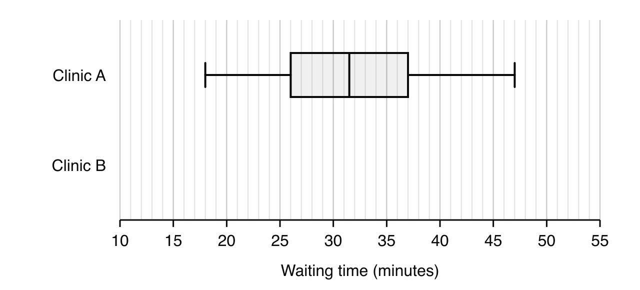
A health authority records the waiting times, in minutes, of 12 randomly chosen patients at each of two clinics, A and B.

Clinic A	18	22	25	27	29	31	32	34	36	38	41	47
Clinic B	12	15	17	19	20	22	23	24	26	28	31	52

The waiting times for clinic A are shown in the following box-and-whisker diagram.

Box-and-whisker diagram for Clinic A on a scale of waiting time from 10 to 55 minutes: minimum 18, lower quartile 26, median 31.5, upper quartile 37, maximum 47. The row for Clinic B is empty.

(a)
For the waiting times at clinic B, write down
(i) the median;
(ii) the lower quartile and the upper quartile.
3 marks
(b)
Show that the waiting time of 52 minutes at clinic B is an outlier.
2 marks
(c)
On the same scale as the diagram, draw a box-and-whisker diagram for the waiting times at clinic B.
3 marks
(d)
Make two comparisons between the waiting times at the two clinics.
2 marks
(e)
The health authority wants to test, at the 5% significance level, whether the mean waiting time at clinic B is less than at clinic A. It assumes that the waiting times at each clinic are normally distributed with equal variances.
Write down the null and alternative hypotheses.
2 marks
(f)
Find the $p$ -value for the test.
2 marks
(g)
State the conclusion of the test. Give a reason for your answer.
2 marks
(h)
With reference to your diagram for clinic B, comment on the assumption that the waiting times at clinic B are normally distributed.
1 mark

Answer it, then compare with the markscheme.Check this one with a free account

Carry on with 4.11 in Augment

With a free account, Augment remembers where you stopped and what you have practiced.

Start free Open 4.11 in Augment

Key terms introduced here

Notes on 4.11 Hypothesis testing

Learning objectives

Introduction

The logic of a hypothesis test

Null and alternative hypotheses

Significance levels and p-values

The decision rule

Critical values

Steps of every test

Observed and expected frequencies

Measuring the discrepancy: the chi-squared statistic

The chi-squared distribution and degrees of freedom

The chi-squared goodness of fit test

By hand and on the GDC: testing a die

GDC procedure for goodness of fit

Given ratios and percentages

Testing a genetic ratio: Mendel's peas

Goodness of fit to a normal model

Contingency tables and the chi-squared test for independence

Expected frequencies under independence

Degrees of freedom for a contingency table

GDC procedure for independence

Interpreting the result

Case study: survival on the Titanic

A full test for independence

The t-test

The idea behind the t-statistic

Assumptions of the pooled t-test

GDC procedure for the t-test

One-tailed and two-tailed tests

Choosing and reporting a test

Exam focus

Practice questions

Summary

Self-check

Questions on 4.11

Markscheme (a)

Markscheme (b)

Markscheme (c)

Markscheme (d)

Markscheme (e)

Markscheme (f)

Markscheme (g)

Markscheme (h)

Carry on with 4.11 in Augment