4.10 Spearman’s rank correlation

Introduction

Many relationships in the real world move in one direction without following a straight line. Richer countries tend to have longer life expectancy, but each extra thousand dollars of income adds less and less; a cup of tea cools quickly at first and then slowly; a pebble shrinks fast near the source of a river and slowly further downstream. Other data exist only as an order, such as two judges' placings of the same divers or a league table. Spearman's rank correlation coefficient measures how consistently two variables move together in such cases, by replacing every value with its position in order and then measuring how closely the two sets of positions agree.

The coefficient is named after the English psychologist Charles Spearman, who introduced it in 1904 in his research in psychology. It is used throughout the sciences, geography and psychology wherever data are ordered, curved or contain an extreme value that would distort Pearson's product-moment correlation coefficient (r).

Ranking data

Ranks

Ranking replaces each value in a data set by its position when the values are put in order. The smallest value is given rank 1, the next smallest rank 2, and so on up to rank $n$ for the largest of $n$ values. The ranks keep the order of the data but lose the sizes of the gaps between values, so the values 3, 4 and 50 have ranks 1, 2 and 3, exactly the same as the values 3, 4 and 5.

Ranking can go in either direction: 1 for the smallest value or 1 for the largest. A league table gives rank 1 to the highest score, while a scientist usually gives rank 1 to the smallest measurement. Either choice works, as long as both variables are ranked in the same direction. Ranking one variable from the smallest and the other from the largest reverses one set of ranks, which changes the sign of the coefficient and turns a positive association into an apparently negative one.

In every column of the table the two ranks add to $n + 1 = 5$, so one row of ranks is the other reversed. Reversing one variable's ranks multiplies the coefficient by $-1$ but does not change its size.

Ordinal data

Some data can be put in order even though the gaps between values have no fixed size. A customer rating of 1 to 5 stars, a finishing position in a race, a grade of A to E, or "strongly disagree" to "strongly agree" on a questionnaire are all of this kind. The step from 4 stars to 5 stars need not mean the same as the step from 1 star to 2 stars, so adding or averaging such values is open to question.

Ordinal data are already ranks, or can be turned into ranks directly. This makes them a natural fit for a rank correlation coefficient. Pearson's $r$ uses the actual sizes of the values, so it needs numerical data measured on a scale with equal steps, called quantitative data. Data that exist only as an order, such as a published league table that gives only positions, can be analysed with $r_s$ but not with $r$.

Tied ranks

When two or more values are equal, they cannot be put in order between themselves, so it would be unfair to give one of them a higher rank than the other. Instead, each tied value receives the mean of the ranks they would have occupied. Two values that would occupy places 4 and 5 both receive rank $\frac{4 + 5}{2} = 4.5$, and the next value receives rank 6. Three values sharing places 2, 3 and 4 all receive rank 3.

Averaging keeps the total of all the ranks the same as for untied data, $1 + 2 + \dots + n = \frac{n(n+1)}{2}$, so the ranks stay centred on the same middle value, $\frac{n+1}{2}$. The rank after a group of ties continues from the last position the group occupied, never from the averaged rank: after two values sharing rank 4.5 (places 4 and 5), the next value is ranked 6, not 5.5 or 5.

The formula works for any number of tied values, because the positions they share are consecutive whole numbers and the mean of consecutive whole numbers is the mean of the first and last.

Spearman's rank correlation coefficient

Pearson's r applied to the ranks

Pearson's $r$ from subtopic 4.4 measures how closely a set of points on a scatter diagram lies to a straight line. Spearman's idea is to apply exactly the same calculation to the ranks instead of to the original values. If one variable always increases when the other increases, then the smallest $x$ is paired with the smallest $y$, the second smallest with the second smallest, and so on, so the rank pairs are $(1, 1), (2, 2), \dots, (n, n)$. These points lie exactly on a straight line, and Pearson's $r$ for them is exactly 1.

Because $r_s$ is a value of Pearson's $r$, it shares the same range and the same reading of its sign.

A positive $r_s$ means that higher ranks of one variable tend to go with higher ranks of the other; a negative $r_s$ means that higher ranks of one variable tend to go with lower ranks of the other; a value near 0 means that the ranks show no consistent pattern.

Monotonic relationships

The relationship that gives $r_s = 1$ does not need to be linear. It only needs one variable to increase whenever the other increases. A relationship like this is called monotonic.

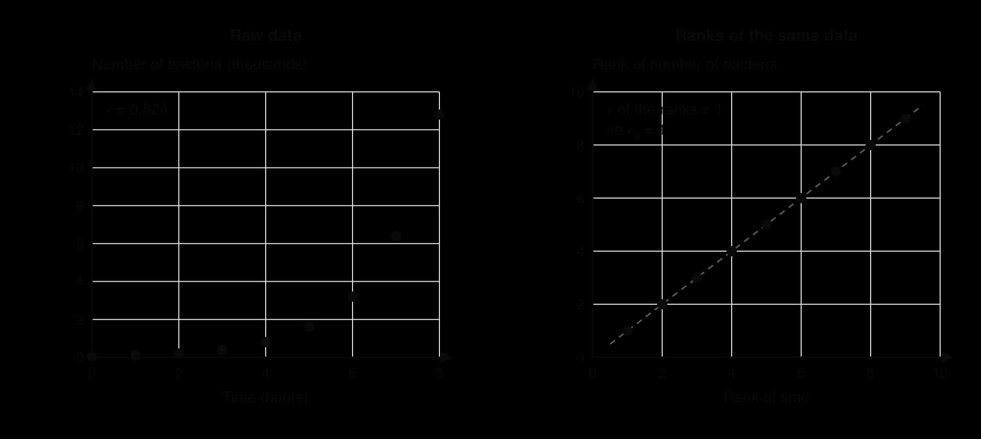
A (hypothetical) culture of bacteria starts with 50 cells and doubles every hour for 8 hours. The counts 50, 100, 200, …, 12,800 curve sharply upwards, so the points are far from a straight line and Pearson's $r$ is only 0.824. The ranks of time and of count, however, are both 1, 2, …, 9 in the same order. The scatter diagram of the ranks of the bacteria data shows nine points exactly on the line through $(1, 1)$ and $(9, 9)$, so $r_s = 1$.

The same reasoning gives the meaning of the extreme values of $r_s$.

A formula for data without ties

When there are no tied ranks, Pearson's $r$ applied to ranks simplifies to a short formula. For each data pair, let $d$ be the difference between the two ranks. Then

where $n$ is the number of pairs. In practice $r_s$ is found with technology, so the formula serves mainly to show how the coefficient behaves. When the rankings are identical, every $d = 0$, so $r_s = 1$. The more the rankings disagree, the larger $\sum d^2$ becomes and the smaller $r_s$ becomes. When one ranking is the reverse of the other, $\sum d^2$ takes its largest possible value, $\frac{n(n^2 - 1)}{3}$, and the formula gives $1 - 2 = -1$.

The simplification relies on the ranks being exactly the whole numbers 1 to $n$. With tied ranks it no longer holds, and the formula gives a slightly different value from Pearson's $r$ of the ranks; the more ties, the larger the difference.

Calculating r_s with a GDC

Every GDC can calculate Pearson's $r$, so the same function gives $r_s$ once the ranks are entered. Most GDCs have no command that ranks data with averaged ties, so the ranks are usually worked out by hand and typed in.

1. Rank the first variable, giving tied values the mean of the positions they share.

2. Rank the second variable in the same direction (rank 1 for the smallest in both, or for the largest in both).

3. Enter the ranks of the first variable in one list and the ranks of the second variable in another, keeping each pair in the same row.

4. Run the linear regression or two-variable statistics function on the two lists of ranks. On a TI-84 Plus CE, STAT → CALC → LinReg(ax+b) shows $r$ once statistics diagnostics are switched on in the MODE screen; on a Casio fx-CG50, MENU → Statistics → CALC → REG → X → ax+b shows $r$.

5. Write down the value of $r$ shown as $r_s$, correct to 3 significant figures.

Spreadsheets can do the ranking too: the function RANK.AVG in common spreadsheet programs gives tied values their average rank, and the correlation function CORREL applied to the two columns of ranks then gives $r_s$.

Interpreting Spearman's rank correlation coefficient

Strength and direction

A value of $r_s$ is described by its sign (positive or negative) and its size (how close it is to 1 or −1). There is no single agreed scale for the size; a commonly used guide is set out in the table, and other sources draw the boundaries slightly differently.

The words used to interpret $r_s$ need care. Pearson's $r$ measures linear correlation between two variables. Spearman's $r_s$ measures the linear correlation between the ranks, and so describes a monotonic association between the variables themselves. A value of $r_s = 0.937$ for income and life expectancy across twelve countries says that richer countries almost always have longer life expectancy; it does not say that life expectancy rises in a straight line with income.

There are two correct ways to interpret $r_s$ in words. The first speaks of association between the variables, for example "there is a strong positive association between practice time and typing speed". The second speaks of correlation between the ranks, for example "there is a strong positive linear correlation between the rank order of practice times and the rank order of typing speeds". Saying "there is strong linear correlation between practice time and typing speed" mixes the two and is wrong, because $r_s$ says nothing about whether the raw data lie near a line.

Agreement between rankings

When both variables are rankings of the same items, such as two judges placing the same competitors, $r_s$ measures how far the two orders agree. A value close to 1 means the judges put the competitors in almost the same order; a value close to −1 means one judge's order is almost the reverse of the other's; a value near 0 means their orders have little in common.

In the diving example, $r_s = 0.922$, so the two judges show strong agreement in the order in which they placed the divers. Agreement between rankings does not mean that the judges gave the same scores: one judge could give every diver exactly one point more than the other and $r_s$ would still be 1, because only the order of the scores enters the calculation.

What r_s does not show

Spearman's coefficient shares the limits of every correlation coefficient. A strong association does not show causation: two variables can rise together because both depend on a third variable, as shoe size and reading age both depend on a child's age. A value of $r_s$ also comes from a sample, so a strong value from very few pairs (four or five, say) can arise by chance. Testing whether a value is large enough to rule out chance needs a critical value or a hypothesis test.

No equation comes from $r_s$, so it cannot be used for prediction. There is no "Spearman regression line": the ranks have lost the sizes of the values, so they cannot turn a value of $x$ into a value of $y$. Predictions are made with the regression line of y on x from subtopic 4.4, and only when the relationship is linear and the correlation is strong.

Choosing between Pearson's r and Spearman's r_s

Linear and monotonic relationships

Pearson's $r$ measures how close the points are to a straight line. It is the right measure when the relationship is linear, and only then. Spearman's $r_s$ measures how consistently the relationship rises or falls, so it suits any monotonic relationship, whether straight or curved. Every linear relationship with a non-zero gradient is monotonic, so for linear data the two coefficients are usually close; for curved monotonic data, $r_s$ is closer to $\pm 1$ than $r$ is.

The four scatter diagrams of ten points each show the main patterns side by side, with both coefficients for each.

The first diagram shows linear data, where both coefficients are about 0.98. In the second, the points rise steeply and then level off: the relationship is perfectly monotonic, so $r_s = 1$, but the curve pulls $r$ down to 0.878. A value of $r = 0.878$ alone would understate how perfectly consistent the pattern is. The third and fourth diagrams show the two main limitations of the coefficients: sensitivity to an outlier, and failure to detect a pattern that changes direction.

Relationships that are not monotonic

Neither coefficient measures a relationship that rises and then falls, or falls and then rises. In the U-shaped diagram, the points follow a clear curve, yet $r = 0.032$ and $r_s = 0.152$, both close to 0. The ranks of $y$ go down and then up again as the ranks of $x$ increase, so there is no consistent direction for either coefficient to measure. A coefficient close to 0 therefore means "no linear relationship" for $r$ and "no monotonic relationship" for $r_s$; it never proves that the variables are unrelated.

Data that exist only as ranks

Pearson's $r$ needs values measured on a numerical scale. When the data are ordinal, such as star ratings, positions in a league table or judges' placings, the sizes of the gaps are unknown and only $r_s$ can be used. Spearman's coefficient is also the natural choice when a question asks about agreement between two people's orderings, because agreement concerns order only.

Appropriateness and limitations of each coefficient

The table brings together what each coefficient measures, when to use it and where it fails.

Spearman's coefficient is not simply "better". Because it keeps only the order of the values, it throws away information. For linear data without outliers, Pearson's $r$ uses the full sizes of the values, measures exactly the relationship that a regression line models, and is the coefficient to report alongside a regression line.

The effect of outliers

Why ranks limit the influence of an outlier

An outlier is a value far from the rest of the data. Pearson's $r$ is calculated from distances from the mean, so one point a long way from the others can pull $r$ a long way from the value given by the rest of the data. Once data are ranked, however, the most extreme value can only be given rank 1 or rank $n$, whatever its size. A value of 25 and a value of 2,500 at the top of a list both receive rank $n$. This caps the influence of an extreme value, so $r_s$ is a robust measure, much less sensitive to outliers than $r$.

The diagram with one outlier among the four relationships shows this. Without the outlier, the ten points lie almost exactly on a line, with $r = 0.999$ and $r_s = 1$. One point recorded as 15 instead of 5 drops $r$ to 0.629, while $r_s$ falls only to 0.818. Raising the outlier further, to 20, drops $r$ to 0.460, yet $r_s$ stays at 0.818, because the point already has the highest rank.

The scatter diagram of the lateness data shows why $r$ falls: seven points lie close to a steep line, and the eighth sits far to the right, well below where that line would go.

Removing a point is not automatically correct. A genuine but extreme value, such as one student who really lives 25 km away, is part of the data; deleting it to improve $r$ misrepresents the situation. An outlier that comes from a recording error should be corrected or removed. Subtopic 4.1 gives the $1.5 \times$ IQR test for deciding whether a value is an outlier: here the distances have $Q_1 = 2.8$ and $Q_3 = 7.05$, so the upper fence is $7.05 + 1.5 \times 4.25 = 13.425$ and 25.0 km is an outlier.

When r_s does not change

A change in a data value leaves $r_s$ unchanged whenever it leaves every rank unchanged. This happens if the value moves without passing or reaching any other value of the same variable. Pearson's $r$ uses the values themselves, so it changes whenever any value changes.

What ranking throws away

The robustness of $r_s$ comes at a price. Ranking treats a gap of 0.1 and a gap of 100 between neighbouring values in exactly the same way. Two data sets with very different patterns of spacing can have identical ranks, and so identical $r_s$, while their values of $r$ differ greatly. When the size of the effect matters (how many extra years of life expectancy go with each extra thousand dollars of income, for example), $r_s$ cannot supply it, and a model fitted to the values is needed.

Case study: the Preston curve

The Preston curve, first described by the demographer Samuel Preston in 1975, links a country's income per person to the life expectancy of its population. Life expectancy rises steeply with income in poorer countries and then levels off in richer ones. The relationship is a classic example of a monotonic but strongly curved pattern.

The table lists twelve countries across the full range of incomes, with GDP per capita measured at purchasing power parity (PPP), which adjusts for differences in prices between countries.

Source: World Bank, World Development Indicators (NY.GDP.PCAP.PP.CD and SP.DYN.LE00.IN), 2023 values, accessed 2026.

The scatter diagram of the twelve countries shows the Preston shape: a steep rise among the poorest countries, then a long, almost flat stretch from Poland to Norway.

Ranking the countries

Ranking both variables from the smallest gives the table of ranks. There are no ties in either variable, so the column of differences $d$ can also be used as a check with the formula for untied ranks.

Ten of the twelve countries have the same rank for income and for life expectancy. Only Bangladesh and Indonesia swap places: Bangladesh has the fourth-lowest income but the seventh-lowest life expectancy, and Indonesia the reverse.

Comparing the two coefficients

Pearson's $r$ for the raw data and Spearman's $r_s$ for the ranks, both from the GDC, are

The formula check gives the same $r_s$, because there are no ties.

The two values describe the data differently. Pearson's $r = 0.719$ suggests only a moderate linear correlation, because the points bend away from any straight line: Norway's income is far larger than Poland's or the United Kingdom's, but its life expectancy is only slightly higher. Spearman's $r_s = 0.937$ shows a strong positive association: across these twelve countries, a higher income almost always goes with a longer life expectancy. Since the pattern is monotonic and curved, $r_s$ is the more appropriate measure.

Interpretation and limitations

The strong association does not show that income alone causes longer lives. Preston himself found that the whole curve moved upwards over the twentieth century, with life expectancy rising at every level of income through better public health, vaccination and medical technology. Some countries lie well below the curve; South Africa, for instance, had a 2023 GDP per capita of about 15.2 thousand international dollars but a life expectancy of only 66.1 years, much lower than other countries with a similar income. The sample of twelve countries was chosen to cover the range of incomes, not at random, so it shows the shape of the relationship rather than estimating a value for all countries. Finally, the ranks do not measure how much life expectancy changes per dollar; that question needs a model fitted to the values, such as one in terms of the logarithm of income, a technique for HL students in subtopic 4.13.

Exam focus

Spearman's rank correlation appears on Papers 1 and 2, usually as the last few parts (4–6 marks) of a longer question that has already asked for Pearson's $r$, a regression line or an outlier check on the same data. The command terms are write down, complete (a table of ranks), find or calculate ($r_s$), interpret, explain (why $r_s$ is unchanged, or why a coefficient is or is not appropriate), state … justify (which coefficient to use) and comment.

The recurring question shapes are:

• complete a table of ranks with one or two tied values missing (one mark for each variable or each missing rank);

• find $r_s$ (usually A2, with follow-through from the candidate's own ranks);

• interpret $r_s$ as association between the variables or agreement between rankings (one mark, lost for "linear correlation" of the raw data);

• explain why $r_s$ does not change when a value is corrected (the rank is the same);

• state which coefficient is more appropriate, with a reason based on the scatter diagram (curved but monotonic, or an outlier present);

• judge agreement between two judges or two tests.

The working to write down is the table of ranks (with averaged ties), the statement that $r_s$ is Pearson's $r$ of the ranks or simply $r_s =$ value, and $r_s$ to 3 significant figures with its sign. Calculator notation and screen labels are not working. No Spearman formula and no rule for tied ranks appear in the formula booklet, so the ranking method has to be known.

Questions on agreement between judges reward two ideas in the interpretation: the strength (strong, moderate, weak) and a reference to the rank order. "The judges strongly agree on the order of the competitors" earns the mark; "the judges give similar scores" does not, because $r_s$ can be 1 even when one judge's scores are all higher.

When a question asks which coefficient to use, the reason must come from the shape of the data: "the scatter diagram is curved but always decreasing, so the relationship is monotonic but not linear" or "there is an outlier, and $r_s$ is less affected by outliers". Vague reasons such as "Spearman is more accurate" earn no marks.

Practice questions

1. Write down the ranks of the values 4.2, 3.8, 5.1, 3.8, 4.7, 5.1, 5.1, 2.9, using rank 1 for the smallest value. [2]

2. State the value of $r_s$ for each data set. [2] (a) $x$: 1, 2, 3, 4, 5, 6 and $y = x^3$. (b) $x$: 1, 2, 3, 4, 5 and $y = \frac{1}{x}$.

3. Two food critics rank the same six restaurants. Critic A ranks them 1, 2, 3, 4, 5, 6 and Critic B ranks the same restaurants 2, 1, 4, 3, 6, 5. Calculate $r_s$ and interpret the result. [3]

4. A kiosk records the hours of sunshine $s$ and the number of ice creams sold $i$ on seven days.

(a) Find the ranks of $s$ and of $i$, using rank 1 for the smallest value. [2] (b) Find $r_s$. [2] (c) Interpret your answer to (b). [1]

5. In question 4, the sunshine on the fifth day was really 11.5 hours, not 10.5 hours. Explain why the value of $r_s$ does not change. [1]

6. For each situation, state whether Pearson's $r$, Spearman's $r_s$ or neither is appropriate, and justify your answer. [6] (a) The heights and arm spans of 30 adults, whose scatter diagram shows points close to a straight line with no outliers. (b) The age and value of 20 cars, where the value falls quickly at first and then more slowly. (c) Engine speed and fuel economy of a car, where fuel economy rises to a maximum and then falls.

7. The data set $x$: 1, 2, …, 10 and $y$: 2.1, 3.0, 4.2, 4.8, 6.1, 7.0, 7.9, 30, 10.1, 10.8 contains one outlier. (a) Find $r$ and $r_s$. [3] (b) The value 30 is a recording error for 9.0. Find $r$

8. A dealer records the age $A$ (years) and the price $P$ (thousand dollars) of ten used cars of the same model.

(a) Find Pearson's $r$. [2] (b) Find the ranks of $A$ and of $P$, using rank 1 for the smallest value. [2] (c) Find $r_s$. [2] (d) The scatter diagram of $P$ against $A$ curves, with the price falling more slowly as the car gets older. State, with a reason, which coefficient is more appropriate, and interpret it. [3]

Summary

• Ranking replaces each value by its position in order; both variables must be ranked in the same direction.

• Tied values each receive the mean of the positions they occupy, and the next value continues from the last position used.

• Spearman's rank correlation coefficient $r_s$ is Pearson's $r$ calculated for the ranks, found with a GDC; $-1 \le r_s \le 1$.

• $r_s = 1$ or $-1$ for any perfectly monotonic relationship, linear or curved; $r_s$ near 0 means no monotonic association.

• Interpret $r_s$ as association between the variables or agreement between rankings, or as linear correlation between the ranks, never as linear correlation of the raw data.

• Pearson's $r$ suits linear relationships between quantitative variables; $r_s$ suits monotonic relationships, ordinal data and rankings; neither suits a relationship that changes direction.

• An outlier can change $r$ greatly but has a limited effect on $r_s$, because its rank is capped at 1 or $n$.

• $r_s$ does not change when a value changes without changing any rank; $r$ changes whenever a value changes.

• Neither coefficient shows causation, and $r_s$ gives no equation for prediction.

Self-check

• To do:

  I can rank a data set from the smallest or from the largest value.

• To do:

  I can give tied values the average of the positions they share and continue the ranking correctly.

• To do:

  I can check a set of ranks by comparing their total with $\frac{n(n+1)}{2}$.

• To do:

  I can find $r_s$ by entering the ranks into the GDC and reading off $r$, not $r^2$.

• To do:

  I can explain why $r_s = 1$ for a curved relationship that always increases.

• To do:

  I can interpret $r_s$ in context using "association" or "agreement between rankings".

• To do:

  I can write a table of ranks as working before giving $r_s$.

• To do:

  I can decide from a scatter diagram whether $r$, $r_s$ or neither is appropriate, with a reason.

• To do:

  I can explain why an outlier affects $r$ more than $r_s$.

• To do:

  I can explain why $r_s$ stays the same when a value changes but its rank does not.

• To do:

  I can explain why $r_s$ cannot be used to make predictions.

• To do:

  I can explain why the shortcut formula with $\sum d^2$ differs from the GDC value when there are ties.

[2]2 marks

0

(b) Enter the ranks of $x$ in one list and the ranks of $y$ in a second list, and use the GDC's linear regression (or two-variable statistics) function on the two lists of ranks. The value of $r$ it gives is $r_s$.

(c) There are no ties, so the formula applies. $\sum d^2 = 0 + 1 + 0 + 0 + 1 + 0 + 0 = 2$ and $n = 7$.

The two methods agree, as they must when there are no ties. The value is close to 1, so there is a strong positive association between practice time and typing speed for these students: students who practise longer tend to type faster.

1

Each row adds to 36, which equals $\frac{8 \times 9}{2}$, so the ranking is consistent.

(b) Pearson's $r$ for the two rows of ranks, from the GDC:

With ties present, the formula $1 - \frac{6\sum d^2}{n(n^2-1)}$ gives $1 - \frac{6 \times 6.5}{8 \times 63} = 0.923$, which differs in the third significant figure. The value from the GDC, Pearson's $r$ of the ranks, is the one to give.

(b) Both values are close to 0, which suggests very weak association. A scatter diagram, however, shows a clear U-shape: electricity use falls as the temperature rises to about 15–20 °C and then rises again. The relationship is neither linear nor monotonic, so neither coefficient is suitable. Both coefficients describe the strength of the relationship as very weak when it is in fact strong but changes direction.

(c) There is a strong negative association between waiting time and satisfaction: customers who wait longer tend to give lower ratings.

The shortcut formula $1 - \frac{6\sum d^2}{n(n^2-1)}$ would give $-0.946$ here, because three pairs of ties break the assumption behind it. Only the GDC value is correct.

(c) Spearman's $r_s$. Every student who lives further away arrived later, so the association is perfectly monotonic. The outlier at 25.0 km, far beyond the other distances, lowers Pearson's $r$ from 0.998 to 0.776, while $r_s$ is unchanged because the outlier still has the highest rank in both variables.

$s = 4$ A1

[2 marks]

(c) Pearson's $r$ for the ranks (M1)

$r_s = -0.994$ $(-0.994029\ldots)$ A1

Accept $0.994$ only if one variable has been ranked in reverse and this is stated. Follow through from their ranks in (b).

[2 marks]

(d) There is a strong negative association between the distance downstream and the mean pebble length (pebbles tend to be smaller further downstream).

OR there is a strong negative linear correlation between the ranks of distance and the ranks of pebble length. A1

Do not accept "strong negative linear correlation between distance and length".

[1 mark]

(e) $r_s$ A1

the relationship is not linear (it is curved), but $L$ never increases as $d$ increases (the relationship is monotonic decreasing) R1

Do not award A1R0.

[2 marks]

(f) 15.0 km is still the greatest distance, so site H keeps rank 8 and none of the ranks change R1

[1 mark]

Total [10 marks]

[2]2 marks