4.9 The normal distribution

Many measured quantities cluster around a central value, with values further from the centre becoming steadily rarer on both sides: the masses of eggs from one farm, the times a commuter takes to reach work, the scores on a well-designed test, the volume of drink a machine puts in a can. The normal distribution is the probability model for this pattern. Its graph is the familiar symmetric bell shape, and two numbers fix it completely: the mean, which locates the centre, and the standard deviation, which sets the spread.

The normal distribution is the most widely used model in statistics. Manufacturers use it to decide how full to fill a pack so that almost none are underweight; psychologists use it to turn test scores into percentiles; engineers use it to set tolerances. Because the normal distribution describes a continuous quantity, probabilities are areas under its curve rather than sums of separate bars, and a graphic display calculator finds those areas.

Continuous random variables

A random variable is discrete when its values can be listed, such as the number of heads in ten coin tosses (subtopic 4.7, Discrete random variables). Many quantities are not like this. A mass, a length, a time or a temperature can take any value in an interval, limited only by how precisely it is measured. The mass of an egg could be 61.2 g, 61.23 g or 61.2347 g; between any two possible values there are infinitely many more.

Probability as area

For continuous data a histogram shows how the values are spread. When the class widths are made smaller and the number of observations grows, the tops of the bars form a smoother and smoother outline. In the limit the outline becomes a curve, and the proportion of values between two numbers $a$ and $b$ becomes the area under the curve between $a$ and $b$.

This gives the two rules every continuous model follows:

• the curve is never below the horizontal axis, because probabilities are never negative;

• the total area under the curve is exactly 1, because the variable is certain to take some value.

The probability of a single value

Because a probability is an area, the probability that a continuous random variable takes one exact value is zero: a vertical line has width 0, so the "area" above a single point is 0.

It follows that including or excluding an endpoint changes nothing. For a continuous $X$, $\mathrm{P}(X < a) = \mathrm{P}(X \le a)$ and $\mathrm{P}(a < X < b) = \mathrm{P}(a \le X \le b)$. This is a real difference from discrete distributions such as the binomial distribution in subtopic 4.8, where $\mathrm{P}(X < 3)$ and $\mathrm{P}(X \le 3)$ are different because $\mathrm{P}(X = 3)$ is not zero.

The normal distribution and the normal curve

A normal distribution is a particular continuous distribution whose curve is a symmetric bell. It has two parameters: the mean $\mu$ and the standard deviation $\sigma$. Every normal curve has the same shape; changing $\mu$ slides it along the axis and changing $\sigma$ stretches or squeezes it.

The notation N(μ, σ²)

The statement $X \sim \mathrm{N}(\mu, \sigma^2)$ is read "$X$ is normally distributed with mean $\mu$ and variance $\sigma^2$". The second number is the variance, the square of the standard deviation (subtopic 4.3, Measures of central tendency and dispersion). Questions usually write the variance as a square so that the standard deviation is easy to read off.

When a question gives $\mathrm{N}(40, 16)$ without a square, the variance is 16 and the standard deviation is $\sqrt{16} = 4$. The GDC always asks for the standard deviation, never the variance.

The normal curve

The graph of the normal distribution is its normal curve. Its height at each value shows how densely the values cluster there: high near the mean, low far from it. The height itself is not a probability. Only areas under the curve are probabilities.

The curve has an equation, but it is not needed in this course: the GDC holds it and works out the areas. Its shape is fixed by $\mu$ and $\sigma$ alone, so a sketch needs only those two numbers.

Why the normal distribution occurs in nature

A quantity tends to be normally distributed when it is the combined result of many small, independent influences, each of which can push the value a little up or a little down. Adult height within one sex and one population depends on hundreds of genes and many environmental factors; the fill of a can depends on tiny variations in pressure, timing and temperature; a repeated measurement in a laboratory is affected by many small sources of error. Most influences partly cancel, so values near the centre are common and values far from it, which need most influences to push the same way, are rare.

A Galton board shows the same effect with falling balls: each ball is knocked left or right at many pins, and the heaps at the bottom form a bell shape. The counts follow a binomial distribution, and as the number of rows grows the binomial bar chart approaches a normal curve.

Natural occurrence and its limits

Calling data "approximately normal" is a judgement made from the data. Real data can never be exactly normal, because the normal curve gives a small positive probability to every value, even negative heights, whereas real heights cannot be negative. The model is useful when those impossible regions have negligible probability and the data's shape is close to a symmetric bell. Typical approximately normal quantities include:

• physical measurements of a single population (heights within a sex, lengths of a species of fish, masses of eggs from one breed);

• measurement errors in repeated measurements of the same quantity;

• quantities produced by a controlled process (fill volumes, component lengths);

• scores on tests that have been constructed to be normal, such as IQ tests.

Quantities that are usually not normal include incomes and house prices (strongly skewed to the right), waiting times that are often short but occasionally very long, and small counts such as the number of goals in a match.

Properties of the normal distribution

Every normal distribution has the same set of properties. They follow from the symmetric bell shape, and many questions can be answered with them alone, without the GDC.

The horizontal axis is an asymptote of the normal curve on both sides. The parts of the curve far from the mean have their own name.

Using symmetry

Symmetry turns one known area into several others. If $X \sim \mathrm{N}(\mu, \sigma^2)$ and $\mathrm{P}(X > \mu + d) = p$, then:

The first line is the mirror image of the given tail. The second subtracts the tail from the half of the area that lies above the mean. The third removes both equal tails from the total area of 1.

Comparing normal curves

Changing the mean moves the whole curve along the axis without changing its shape. Changing the standard deviation changes the shape: a larger $\sigma$ gives a wider, flatter curve, and a smaller $\sigma$ gives a narrower, taller one. The height must change with the width because the total area always stays 1.

The curves of A and B both peak at 20, but B is half as tall and twice as wide because its standard deviation is twice as large. C is a copy of A moved 8 units to the right. These two effects are enough to match any set of normal curves to their parameters: first sort the curves by where they peak (the means), then by how wide they are (the standard deviations).

The empirical rule

The proportion of a normal distribution within a given number of standard deviations of the mean is the same for every normal distribution, whatever $\mu$ and $\sigma$ are. This is because every normal curve is the same shape, stretched by $\sigma$ and moved by $\mu$. Three of these proportions are worth knowing by heart.

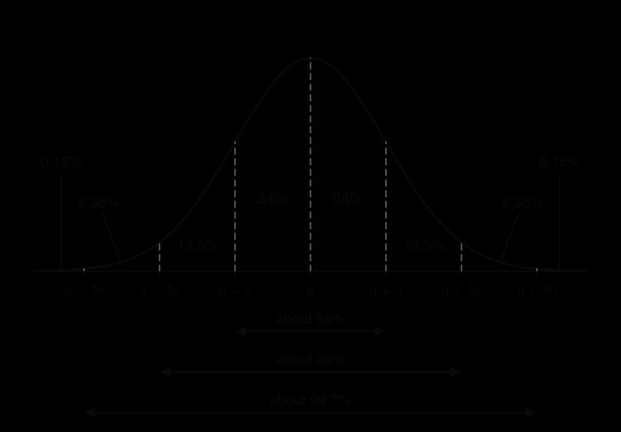
The band percentages in the diagram of the empirical rule come from the three headline figures and symmetry. Half of 68% gives 34% between $\mu$ and $\mu + \sigma$. The band from $\sigma$ to $2\sigma$ above the mean holds half of $95\% - 68\%$, which is 13.5%. The band from $2\sigma$ to $3\sigma$ holds half of $99.7\% - 95\%$, which is 2.35%. What remains beyond $3\sigma$ on each side is half of 0.3%, which is 0.15%.

The percentages in the empirical rule are rounded. The GDC gives the exact areas within one, two and three standard deviations as 0.6827, 0.9545 and 0.9973. The rule is for quick estimates, checks and sketches; probabilities asked for in a question are found with the GDC unless the question asks for the rule.

IQ scores and the empirical rule

Modern intelligence tests convert raw scores so that, in the population the test was designed for, IQ scores follow a normal distribution with mean 100 and standard deviation 15. One standard deviation either side of the mean is 85 to 115, so about two-thirds of people (68%) score in that range. About 95% score between 70 and 130, which leaves about 2.5% above 130 and 2.5% below 70. The exact normal area above 130 is 2.28%, close to the rule's estimate.

The difference in part (c) is small here, but it grows in relative terms further into the tails. Beyond three standard deviations the rule's 0.15% and the exact 0.135% differ by about 11%, which matters when large numbers of items or people are involved.

Diagrammatic representation

A sketch makes every normal probability calculation clearer: it shows which region is wanted and gives a quick check on the size of the answer. A good sketch of a normal curve takes seconds to draw and has five features.

1. Draw a horizontal axis and a symmetric bell curve that approaches the axis on both sides without touching it.

2. Mark the mean $\mu$ on the axis directly below the peak, with its value.

3. Indicate the spread: mark $\mu - \sigma$ and $\mu + \sigma$ with their values, at the points where the curve changes from bending down to bending up.

4. Draw a vertical line at each value in the question, on the correct side of the mean and roughly in proportion, and label it with its value.

5. Shade the region whose area is the probability required, and label the area if it is known.

A value less than $\mu - 3\sigma$ or more than $\mu + 3\sigma$ should sit where the curve is almost on the axis; a value inside $\mu \pm \sigma$ should sit on the steep part of the curve.

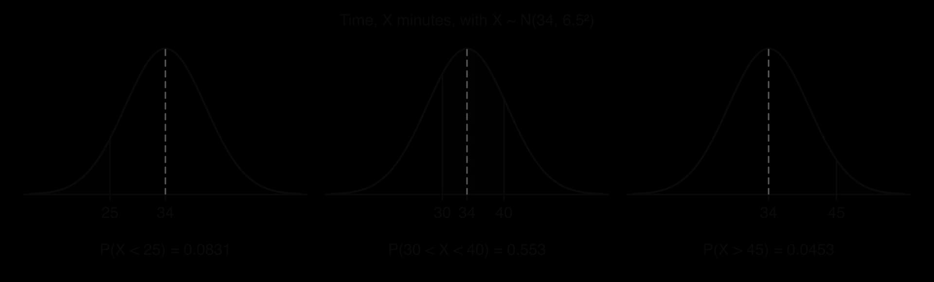
The three sketches of commuting times show the only three shapes of region that occur: a lower tail $\mathrm{P}(X < a)$, a region between two values $\mathrm{P}(a < X < b)$, and an upper tail $\mathrm{P}(X > b)$. Any other region, such as "less than 25 or more than 45", is a combination of these.

Normal probability calculations

A probability for a normal variable is an area under the normal curve. There is no simple formula for these areas, so they are found with technology. The GDC's normal cumulative probability function takes four inputs: the lower bound, the upper bound, the mean and the standard deviation.

The GDC method

To find $\mathrm{P}(a < X < b)$ for $X \sim \mathrm{N}(\mu, \sigma^2)$:

1. Open the normal cumulative distribution function. On a TI-84 Plus CE: 2nd VARS (DISTR) → normalcdf(. On a Casio fx-CG50: MENU → Statistics → DIST → NORM → Ncd. On a TI-Nspire: menu → Statistics → Distributions → Normal Cdf.

2. Enter the lower bound $a$, the upper bound $b$, the mean $\mu$ and the standard deviation $\sigma$.

3. For a lower tail $\mathrm{P}(X < b)$, use a lower bound far below the mean, such as $-10^{99}$; for an upper tail $\mathrm{P}(X > a)$, use an upper bound far above it, such as $10^{99}$.

The open bound only has to be so far from the mean that the area beyond it is negligible. A bound of $\mu \pm 10\sigma$ gives the same answer to many decimal places; a bound of 0 is a common choice for lengths or masses, and is fine when 0 is several standard deviations below the mean.

What to write down

The GDC does the calculation, so the written working records the model and the probability statement in mathematical notation rather than calculator syntax such as normalcdf(-1E99, 25, 34, 6.5). A complete answer states the distribution, the probability statement and its value:

with the region sketched if there is any doubt. Give the answer to three significant figures unless the question asks for a different accuracy, and keep the full GDC value for any later part.

Complements and "at least"

Sometimes a question is easier through its complement. Because the total area is 1:

Wording maps onto inequalities in the usual way: "at least 40" is $X \ge 40$, "at most 40" is $X \le 40$, "more than" is $>$ and "less than" is $<$. For a continuous variable the strict and weak forms give the same answer, so the only thing that matters is the direction. A region outside an interval, such as "less than 25 or more than 45", is the sum of the two tails, or 1 minus the area between.

Expected numbers

When a group of $n$ items or people is drawn from the population, the expected number in a region is $n$ times the probability of the region. This is the expected number from subtopic 4.5.

An expected number is an average over many groups, so it need not be a whole number. Give it to three significant figures unless the question asks for a whole number, in which case round sensibly and state the rounding.

Normal probabilities combined with other probability rules

Once a normal probability is known, it behaves like any other probability. It can be combined with the rules of subtopic 4.6, Combined events, and used as the probability of success in a binomial distribution.

• Several items: if items are independent, the probability that two items both lie in a region is the product of their probabilities.

• Conditional probability: the conditional probability of one region given another is the area of the overlap divided by the area of the given region.

• Counting successes: if $n$ independent items each lie in a region with probability $p$, the number that do is $\mathrm{B}(n, p)$.

Inverse normal calculations

A normal probability question gives a value and asks for an area. An inverse normal question does the opposite: it gives an area and asks for the value that cuts it off. Typical contexts are "the heaviest 2% of bags are rejected: find the rejection mass", "the slowest 15% of runners take longer than $k$ minutes", or "find the 90th percentile".

The GDC method and the left-area convention

The GDC's inverse normal function needs the area, the mean and the standard deviation. By default it treats the area as the area to the left of $k$: it solves $\mathrm{P}(X < k) = \text{area}$.

1. Write the probability statement from the question: $\mathrm{P}(X < k) = p$ or $\mathrm{P}(X > k) = p$.

2. If the statement is an upper tail $\mathrm{P}(X > k) = p$, either change it to the left area $\mathrm{P}(X < k) = 1 - p$, or set the GDC's tail option to the right where it has one.

3. Open the inverse normal function. On a TI-84 Plus CE: 2nd VARS (DISTR) → invNorm(. On a Casio fx-CG50: MENU → Statistics → DIST → NORM → InvN, with Tail set to Left, Right or Central. On a TI-Nspire: menu → Statistics → Distributions → Inverse Normal.

4. Enter the area, $\mu$ and $\sigma$, and read off $k$.

5. Check the answer against a sketch: an area of less than 0.5 to the left of $k$ puts $k$ below the mean.

The written working is the probability statement and the answer, for example "$\mathrm{P}(X > k) = 0.05$, so $k = 85.2$", with a sketch of the region if the statement could be misread.

Central areas

A question may ask for the interval, symmetric about the mean, that contains a given proportion of the values: "the middle 90% of IQ scores". Symmetry splits the remaining area equally between the two tails.

The lower end of the interval has left area 0.05 and the upper end has left area 0.95. Some GDCs do this directly with a central tail option, which returns both ends.

An area between a known value and an unknown value

The hardest inverse normal questions give an area that is neither a tail nor centred on the mean. For example, "60% of loaves have masses between $k$ and 262 g". The inverse normal function only accepts a left area, so the given area has to be turned into the area to the left of $k$.

The method uses the known boundary. First find the area to the left of the known value with the normal probability function. Then subtract the given area: what remains is the area to the left of $k$.

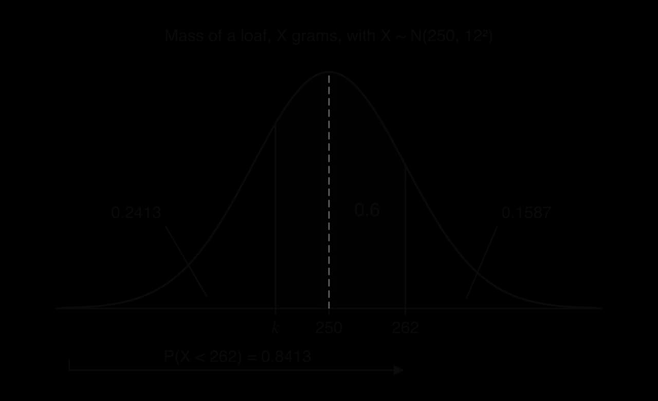
The diagram of loaf masses shows why the subtraction works: the area to the left of 262 is made of two pieces, the shaded 0.6 and the unshaded area to the left of $k$.

Percentiles, quartiles and the interquartile range

A percentile of a normal distribution is an inverse normal value: the 90th percentile is the value $k$ with $\mathrm{P}(X < k) = 0.9$. In particular:

• the median is the 50th percentile, which is $\mu$ by symmetry;

• the lower quartile $Q_1$ has $\mathrm{P}(X < Q_1) = 0.25$;

• the upper quartile $Q_3$ has $\mathrm{P}(X < Q_3) = 0.75$;

• the interquartile range is $Q_3 - Q_1$, and by symmetry it equals $2(Q_3 - \mu)$

When a normal model is appropriate

A normal model is a choice, and it should be checked against the data and the context before its probabilities are trusted. Three checks help.

• Shape: a histogram of the data should be roughly symmetric and bell-shaped, with one peak; a box-and-whisker diagram should be roughly symmetric, with the median near the middle of the box and whiskers of similar length (subtopic 4.2, Presenting data).

• Centre: the mean and the median of the data should be close, since they are equal for a normal distribution.

• Spread: about 68% of the data should lie within one standard deviation of the mean and about 95% within two.

The context matters as well. A model with mean 5 minutes and standard deviation 3 minutes for a waiting time gives $\mathrm{P}(X < 0) = 0.048$, so nearly 5% of waits would be negative. Negative waiting times are impossible, so the model is unsuitable. A variable that is a small count, such as the number of cars in a driveway, is discrete and has only a few values, so a continuous bell curve is a poor description.

Heavy tails

The most serious misuse of the normal distribution is applying it to quantities whose extreme values are much more frequent than the model predicts. Such distributions are said to have heavy tails. Daily changes in share prices are a well-known example. On 19 October 1987, "Black Monday", the Dow Jones Industrial Average fell by 22.6% in a single day. Under a normal model with mean 0 and a standard deviation of about 1 percentage point (an illustrative value for a typical daily change), a fall of that size is more than 22 standard deviations from the mean, with a probability smaller than $10^{-100}$. Under the model such a fall is practically impossible, yet it happened, so a normal model of daily price changes underestimates the risk of extreme losses.

Case study: Filling packs under the average quantity rules

Packed food sold in the UK and the European Union with the ℮-mark next to its stated quantity must meet three "packers' rules". The average contents of a batch must be at least the nominal quantity. The proportion of packs that are short by more than the tolerable negative error (TNE) must be small, in general no more than 2.5%. No pack may be short by more than twice the TNE. For a 500 g pack the TNE is 15 g, so the limits are 485 g and 470 g.

Source: Business Companion (UK Trading Standards), "Packaged goods: average quantity", 2026; Wikipedia, "Estimated sign", 2026.

The machines in this case study are hypothetical. Suppose a factory has two machines filling 500 g packs, and fill masses are normally distributed. Machine A has mean 500 g and standard deviation 6 g; machine B has mean 500 g and standard deviation 9 g. Both machines meet the first rule, because their mean is the nominal 500 g. The second rule depends on the spread.

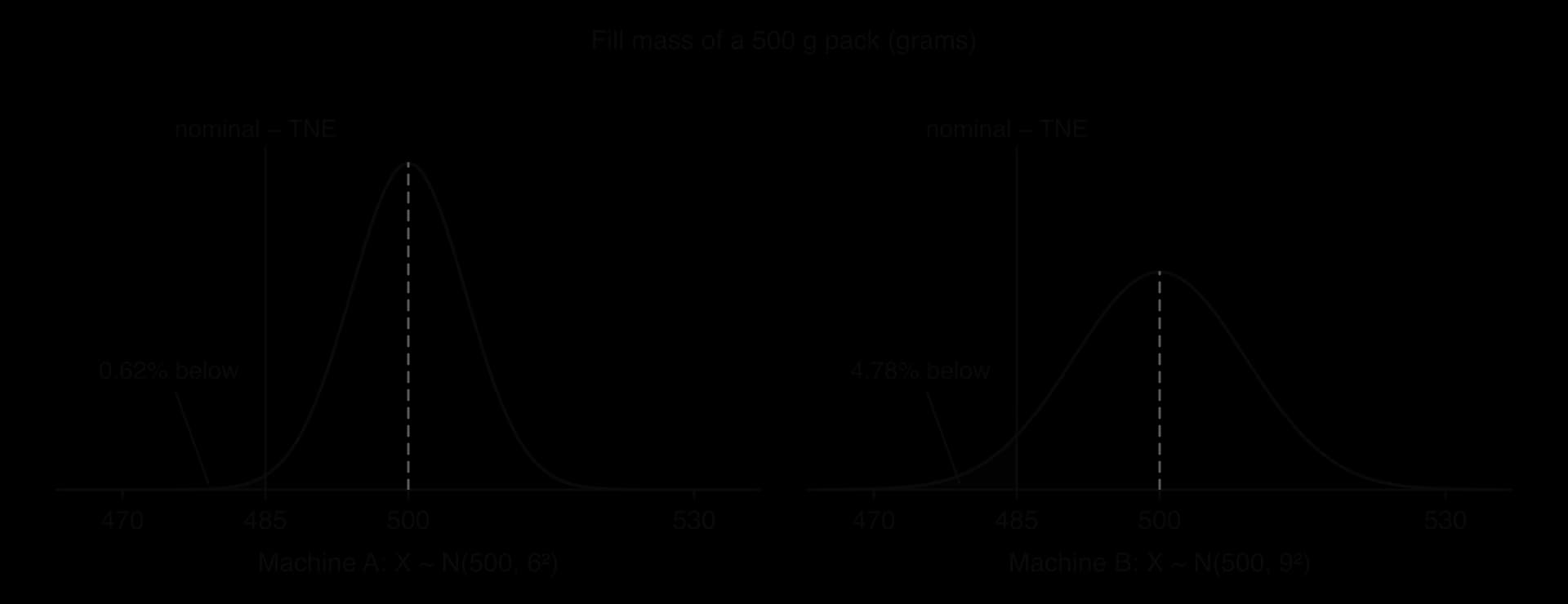
For machine A, $X \sim \mathrm{N}(500, 6^2)$, the GDC gives $\mathrm{P}(X < 485) = 0.00621$, so about 0.62% of packs are short by more than the TNE, well under 2.5%. The rule is met. For machine B, $X \sim \mathrm{N}(500, 9^2)$, $\mathrm{P}(X < 485) = 0.0478$, so about 4.78% of packs are more than 15 g short. The rule fails, even though the average is correct.

The comparison of the two machines shows the role of each parameter. The mean controls whether the average is right; the standard deviation controls how many packs stray into the lower tail. Machine B can meet the rule in two ways: reduce the spread (better maintenance or a better machine) or raise the mean so that the whole curve moves away from 485 g.

Raising the mean to 504 g brings the proportion below 2.5%, but every pack then holds 4 g of product on average that the customer receives free. Over a million packs that is 4 tonnes of product. Inverse normal calculations give the same picture from the other direction: for machine A, the 2.5th percentile of fill mass is 488.2 g, above the 485 g limit; for machine B with mean 500 g it is 482.4 g, below it.

The third rule is a check on the extreme lower tail. For machine B with mean 500 g, $\mathrm{P}(X < 470) = 0.00043$, about 4 packs in 10,000. Packs that light must not carry the ℮-mark at all, so the factory checkweighs and removes them. The normal model gives a small but non-zero number here, and that number is the kind of tail estimate that should be checked against real data, because a fault on the line can produce more very light packs than a normal model predicts.

Exam focus

Normal distribution questions appear very often on Paper 1, as short questions of 4–7 marks, and as parts of Paper 2 questions where they are combined with expected numbers, conditional probability, the binomial distribution or a chi-squared goodness of fit test. The contexts are measurements: masses of products, lengths, times, scores. The command terms are sketch (a labelled bell curve with the region shaded), write down (a value from symmetry with no working, such as $\mathrm{P}(X > \mu) = 0.5$), find and calculate (a GDC probability with its probability statement), estimate or determine (an expected number), and find the value of $k$ (an inverse normal value).

The marks follow a standard pattern. A method mark is awarded for a correct probability statement, such as $\mathrm{P}(X < 6.5)$ or $\mathrm{P}(X > k) = 0.02$, or for a sketch with the correct region shaded and labelled; the answer mark is for the value. For an expected number, the method mark is for multiplying the correct probability by the group size.

The small-egg boundary in part (c) is exactly two standard deviations below the mean, so the empirical rule gives a quick check: about 2.5% of eggs are small, and $360 \times 0.025 = 9$, close to the GDC answer of 8.19. In part (f), every large egg is also "not small", so the overlap of the two events is simply "large".

Questions often set the accuracy explicitly, for example "correct to four decimal places" for probabilities that will be used in a later chi-squared test, or "correct to four significant figures" for expected frequencies. Follow the instruction exactly; otherwise use three significant figures and keep the full GDC value for later parts.

Practice questions

1. The random variable $X$ is normally distributed with $X \sim \mathrm{N}(18, 2.5^2)$. Write down $\mathrm{P}(X > 18)$. [1]

2. The heights of sunflowers in a field are normally distributed with mean 210 cm and standard deviation 15 cm. Use the empirical rule to estimate the percentage of sunflowers between 195 cm and 240 cm tall. [2]

3. The random variable $Y$ is normally distributed with mean 50. Given that $\mathrm{P}(Y < 44) = 0.3$, find $\mathrm{P}(44 < Y < 56)$

4. The lifetimes of a type of light bulb are normally distributed with mean 1200 hours and standard deviation 80 hours. (a) Find the probability that a bulb lasts less than 1050 hours. [2] (b) Find the probability that a bulb lasts between 1100 and 1300 hours. [2] (c) A hotel installs 400 of these bulbs. Estimate the number that last more than 1350 hours. [3]

5. The time taken to solve a puzzle is normally distributed with mean 14.2 minutes and standard deviation 3.1 minutes. The slowest 15% of solvers take longer than $k$ minutes. Find $k$. [3]

6. The heights of adult women in a town are modelled by $\mathrm{N}(1.65, 0.07^2)$ metres. Find the interval, symmetric about the mean, that contains the middle 80% of heights. [3]

7. A machine fills cans with volumes normally distributed with mean 330 ml and standard deviation 4 ml. 70% of cans contain between $k$ ml and 334 ml. Find $k$. [4]

8. The random variable $W$ is normally distributed with mean 40 and standard deviation 6. Estimate the interquartile range of $W$. [3]

9. The times for a runner's 5 km training runs are modelled by $\mathrm{N}(55, 4^2)$ minutes. The runs are independent. (a) Find the probability that a run takes less than 60 minutes. [2] (b) Find the probability that exactly 6 of the next 8 runs take less than 60 minutes. [3]

10. A café models the time its customers wait for their food by $\mathrm{N}(7, 4^2)$ minutes. Calculate $\mathrm{P}(X < 0)$ and hence comment on the suitability of the model. [3]

Summary

• A continuous random variable takes any value in an interval; its probabilities are areas under a curve, so $\mathrm{P}(X = a) = 0$ and $<$ and $\le$ give the same probability.

• $X \sim \mathrm{N}(\mu, \sigma^2)$ is the normal distribution with mean $\mu$ and variance $\sigma^2$; the GDC needs the standard deviation $\sigma$.

• The normal curve is bell-shaped and symmetric about $\mu$; mean = median = mode; total area 1; $\mathrm{P}(X > \mu) = 0.5$; equal distances from $\mu$ cut off equal tails.

• Increasing $\mu$ moves the curve to the right; increasing $\sigma$ makes it wider and lower.

• Empirical rule: about 68%, 95% and 99.7% of values lie within one, two and three standard deviations of the mean (bands of 34%, 13.5%, 2.35% and 0.15%).

• Normal probabilities come from the GDC's normal cumulative function (lower bound, upper bound, $\mu$, $\sigma$); write the distribution and the probability statement, not calculator syntax.

• Expected number in a region = $n \times$ probability of the region; normal probabilities can be multiplied for independent items, used in conditional probabilities, and used as $p$ in a binomial distribution.

• Inverse normal values come from the GDC's inverse normal function, which uses the area to the left of $k$; convert an upper tail with $1 - p$, split a central area equally between two tails, and build the left area from a known boundary for a region between a known value and $k$.

• A normal model needs data that are roughly symmetric and bell-shaped, and is unreliable in heavy-tailed or strongly skewed contexts.

Self-check

• To do:

  I can explain why $\mathrm{P}(X = a) = 0$ for a continuous random variable.

• To do:

  I can read $\mu$, $\sigma$ and $\sigma^2$ from $\mathrm{N}(\mu, \sigma^2)$, including when the variance is not written as a square.

• To do:

  I can list the properties of the normal curve and use symmetry to find probabilities without a GDC.

• To do:

  I can match normal curves to their means and standard deviations.

• To do:

  I can state the empirical rule and split it into bands of 34%, 13.5%, 2.35% and 0.15%.

• To do:

  I can sketch a normal curve with the mean, $\mu \pm \sigma$, the boundary values and the shaded region labelled.

• To do:

  I can find $\mathrm{P}(X < b)$, $\mathrm{P}(X > a)$ and $\mathrm{P}(a < X < b)$

• To do:

  I can calculate an expected number from a normal probability, and estimate a group size from an observed number.

• To do:

  I can combine a normal probability with independence, conditional probability and the binomial distribution.

• To do:

  I can find $k$ from $\mathrm{P}(X < k) = p$ and from $\mathrm{P}(X > k) = p$

• To do:

  I can find the interval holding the middle given percentage of a normal distribution.

• To do:

  I can find $k$ when the given area lies between $k$ and a known value.

• To do:

  I can find the quartiles, the interquartile range and percentiles of a normal distribution.

• To do:

  I can judge whether a normal model suits a context, and explain how heavy tails or skew make it misleading.

Write down the modal class.

[1]1 mark

(c) Removing both tails from the total area:

(d) The interval from 30 to 34 is half of the interval in (c), because the region is symmetric about 30:

As a check, $0.5 - 0.18 = 0.32$.

GDC inverse normal: area $0.241344\ldots$, $\mu = 250$, $\sigma = 12$, giving $k = 241.576\ldots$

$k = 242$ g (3 s.f.) A1

Check: $k$ is below the mean and $\mathrm{P}(241.58 < X < 262) = 0.600$ on the GDC.

$\mathrm{P}(X < Q_3) = 0.75$ gives $Q_3 = 110.117\ldots = 110$

(b) Using the unrounded quartiles:

(c) The fences are

GDC: $\mathrm{P}(X < 59.53\ldots) = 0.003488\ldots$, and by symmetry the same area lies above 140.47.

About 0.7% of a normal population counts as an outlier under the $1.5 \times \text{IQR}$ rule, so a few outliers in a large normal data set are expected and are not evidence of errors.

[2]2 marks

[2]2 marks