3.16 Tree and cycle algorithms

Learning objectives

• Determine whether a sequence of edges is a walk, trail, path, circuit or cycle.

• Determine, with a reason based on vertex degrees, whether a graph has an Eulerian trail or an Eulerian circuit, and write down one when it exists.

• Find Hamiltonian paths and cycles, and explain why a given graph has none.

• Use Kruskal's algorithm and Prim's algorithm to find a minimum spanning tree, showing the order in which edges are chosen.

• Use Prim's algorithm on a weighted adjacency table (the matrix method).

• Use the Chinese postman algorithm to find the shortest route along every edge of a graph with up to four odd vertices, and explain why the algorithm works.

• Construct a table of least distances to turn a practical travelling salesman problem into the classical problem.

• Use the nearest neighbour algorithm to find an upper bound, and the deleted vertex algorithm to find a lower bound, for the travelling salesman problem.

• Interpret upper and lower bounds and justify the choice of algorithm for a route-planning problem.

Introduction

A council gritting lorry has to drive along every road in a town after a frost. A delivery van has to call at twenty shops and return to its depot. An engineer has to connect a set of buildings with cable using as little cable as possible. Each of these problems is set on a weighted graph, and each has a standard algorithm that either solves it exactly or gives a guaranteed range for the best answer. The algorithms fall into two families: those that build trees (minimum spanning trees) and those that build cycles or closed routes (the Chinese postman and travelling salesman problems).

Subtopic 3.14, Graph theory, set up the vocabulary of vertices, edges, degrees and weights, and subtopic 3.15, Adjacency matrices, introduced walks and weighted adjacency tables. Tree and cycle algorithms put that vocabulary to work on routing and network design problems from real life.

Walks, trails, paths, circuits and cycles

A walk is a sequence of edges in which each edge starts where the previous one ended. Vertices and edges may be repeated as often as necessary. Routes in real problems usually come with restrictions, such as "never drive along the same road twice" or "never visit the same town twice", and each restriction gives a special kind of walk with its own name.

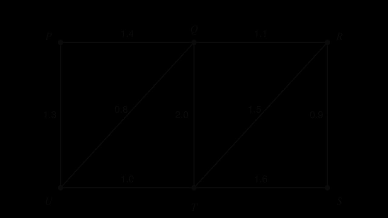
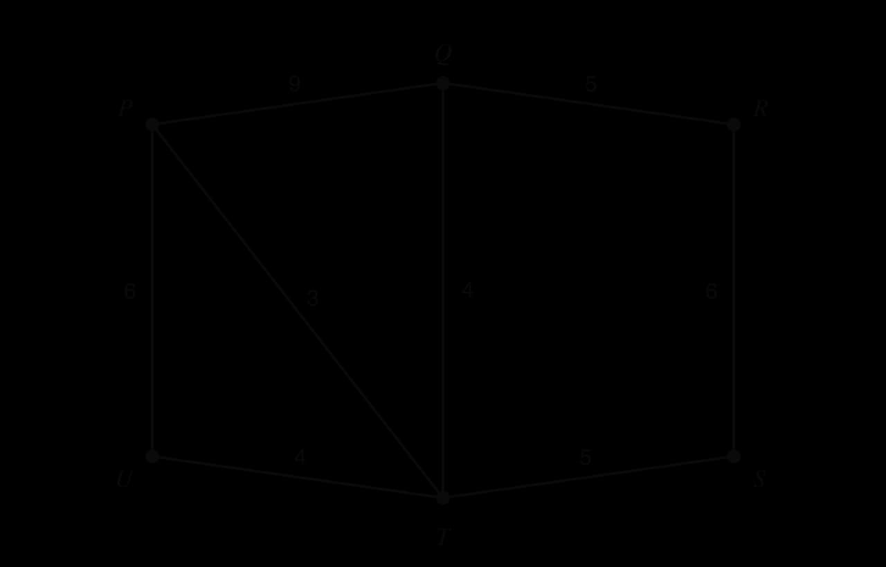
The graph of six road junctions P to U, with distances in kilometres, is the running example for routes. Vertex T has degree 4, P and Q have degree 3, and R, S and U have degree 2.

Open routes: trails and paths

The first restriction forbids repeated edges. In the junction graph, P → Q → T → P → U is allowed under this rule even though it passes through P twice, because each road is used once.

A stricter restriction forbids repeated vertices. If no vertex is repeated then no edge can be repeated either, because using an edge a second time means arriving at its end vertex a second time. Every path is therefore a trail, but not every trail is a path.

Closed routes: circuits and cycles

A route that returns to its starting vertex is called closed. The closed versions of trails and paths have their own names. A circuit may pass through a vertex several times, as long as it never uses the same edge twice.

A cycle is the closed version of a path. The only vertex allowed to appear twice is the start, which is also the end. In the junction graph, P → Q → T → P is a cycle of three edges and P → Q → R → S → T → U → P is a cycle through all six vertices.

The five names form a hierarchy, summarised in the table. Each row after the first adds a restriction to an earlier row.

Every cycle is a circuit, every circuit is a trail, and every trail is a walk. Similarly, every path is a trail. The inclusions run one way only: any path also counts as a trail, but a trail that revisits a vertex is never a path.

Eulerian trails and circuits

A postal worker, a road sweeper or a snowplough driver would ideally travel along every edge exactly once, so that no street is missed and none is covered twice. Such routes are named after Leonhard Euler, whose 1736 analysis of the bridges of Königsberg is usually counted as the start of graph theory.

When the route must also return to its start, the trail becomes a circuit.

Why degrees decide the answer

Every time an Eulerian route passes through a vertex, it arrives along one edge and leaves along a different edge. Each visit therefore uses up two of the edges at that vertex. If the route is a circuit, the start vertex is no different: the first edge leaving it is paired with the last edge arriving back. All of a vertex's edges are used up in pairs, so every vertex must have even degree.

For an Eulerian trail that is not closed, the start and finish vertices are the exceptions. The start vertex has one unpaired edge (the first one leaving) and the finish vertex has one unpaired edge (the last one arriving), so those two vertices have odd degree and all others have even degree. A graph with exactly one odd vertex cannot exist, because the sum of the degrees is twice the number of edges and so is even; the number of odd vertices is always even.

Euler stated, and Carl Hierholzer later proved, that these conditions are also enough: in a connected graph that satisfies them, the route always exists. The result gives two tests, stated for a connected graph.

In the second case the trail must start at one odd vertex and finish at the other. With four or more odd vertices, neither an Eulerian trail nor an Eulerian circuit exists.

A graph that falls one step short has its own name. It can be drawn without lifting the pen but not without finishing in a different place from the start.

Königsberg revisited

The city of Königsberg (now Kaliningrad) was built around two islands in the River Pregel, joined to each other and to the two river banks by seven bridges. Taking each land mass as a vertex and each bridge as an edge gives a graph with multiple edges. The Kneiphof island has five bridges and each of the other three land masses has three.

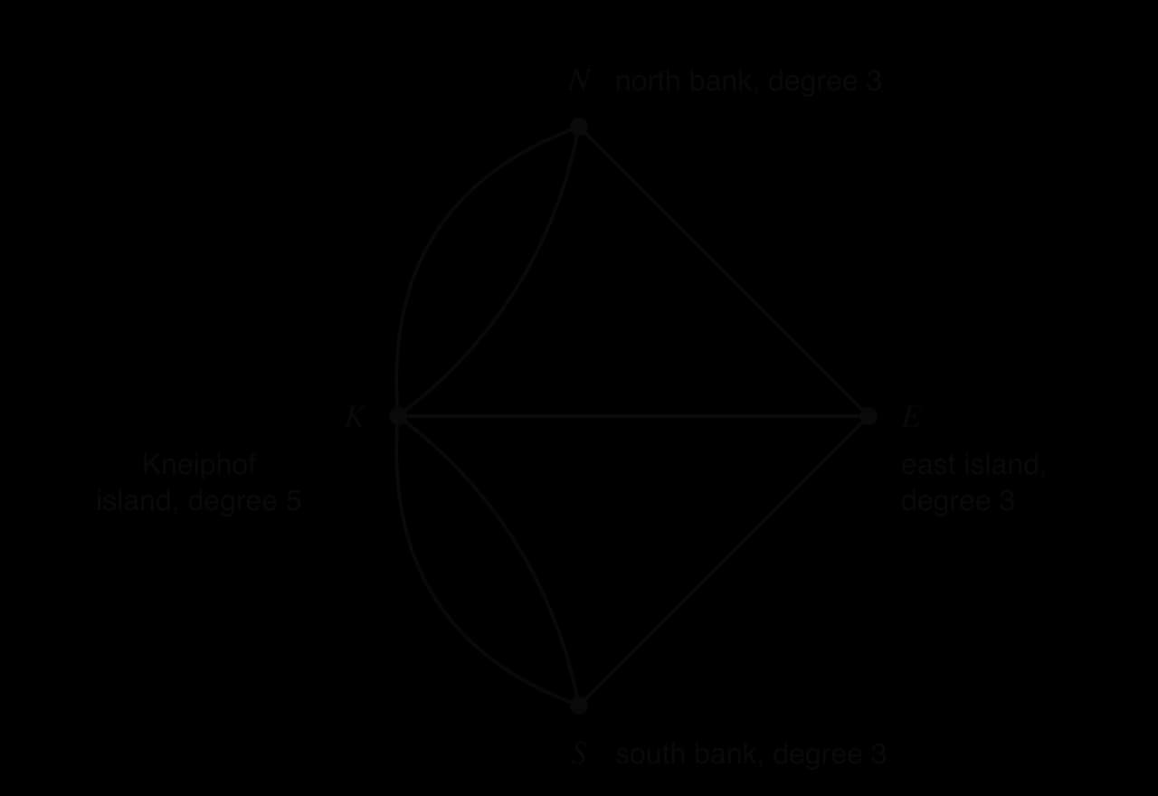
All four vertices are odd, so the graph has neither an Eulerian circuit nor an Eulerian trail, and no walk crosses every bridge exactly once, wherever it starts. The same degree count shows how few repeats are needed. Crossing one bridge a second time acts like an extra edge: a second crossing between N and K makes N degree 4 and K degree 6, leaving only S and E odd, so a walk from S to E that crosses that bridge twice and every other bridge once does exist. A walk that returns to its starting point needs every vertex even, so it must repeat at least two bridges, for example the bridge between N and E and one of the bridges between K and S. Choosing the repeats so that the extra distance is as small as possible is the Chinese postman problem.

YouTube

Finding an Eulerian trail or circuit

Once the degree test says a route exists, it can be found by trial, using two rules.

1. For a trail, start at one of the two odd vertices; for a circuit, start anywhere.

2. At each vertex, choose any unused edge, but avoid an edge whose removal would cut off edges that have not been used yet (do not "burn the bridge" back to unvisited parts of the graph unless no other edge is left).

Cross off each edge as it is used. The route is finished when every edge has been crossed off, and it should end at the second odd vertex (trail) or back at the start (circuit). Small graphs in practice rarely need more than one or two attempts.

Hamiltonian paths and cycles

Eulerian routes are about edges. In many routing problems only the vertices matter: a sales representative must visit every client and a tour must stop at every attraction, whichever roads are left unused. Routes of this kind are named after William Rowan Hamilton, who studied cycles through the corners of a dodecahedron.

Closing a Hamiltonian path with one more edge, back to the start, gives a cycle through every vertex. The two Hamiltonian ideas match the two Eulerian ideas, with vertices in place of edges.

Reasoning about Hamiltonian cycles

There is no simple test, like Euler's degree test, that decides whether a graph has a Hamiltonian cycle. Each graph has to be reasoned about on its own, using facts like these.

• A vertex of degree 1 rules out a Hamiltonian cycle: a cycle must arrive at and leave every vertex along two different edges.

• At a vertex of degree 2, a Hamiltonian cycle must use both of its edges.

• If two vertices of degree 2 share the same two neighbours, a cycle would have to use all four of those edges, which close a cycle of length 4; unless those four vertices are the whole graph, no Hamiltonian cycle exists.

• If removing one vertex splits the graph into two pieces, no Hamiltonian cycle exists: a cycle leaving one piece must come back through that same vertex, visiting it twice.

A Hamiltonian cycle and an Eulerian circuit are different objects. The Hamiltonian cycle P → Q → R → S → T → U → P in the junction graph leaves out the edges QT and PT, so it is not an Eulerian circuit. Odd and even degrees give no information about Hamiltonian cycles: a graph with many odd vertices may have one, and a graph with all vertices even may not.

Counting Hamiltonian cycles in a complete graph

In a complete graph $K_n$ every pair of vertices is joined, so every ordering of the vertices gives a Hamiltonian cycle. Fix the starting vertex: the remaining $n - 1$ vertices can be visited in $(n - 1)!$ orders. Each cycle is counted twice, once in each direction (A → B → C → D → A is the same set of edges as A → D → C → B → A), so the number of distinct Hamiltonian cycles is

For $K_5$ this is $\frac{4!}{2} = 12$, and for $K_{10}$

Spanning trees and minimum spanning trees

A tree is a connected graph with no cycles, and a subgraph is part of a graph made from some of its vertices and edges. A tree on $n$ vertices always has exactly $n - 1$ edges: starting from one vertex, each new edge must bring in exactly one new vertex, because an edge between two vertices already in the tree would close a cycle.

A spanning tree links every vertex to every other, through some route, while using no redundant edges. Removing any edge from a spanning tree disconnects it, and adding any edge creates a cycle. A connected graph usually has many spanning trees, and in a weighted graph they have different total weights.

Minimum spanning trees answer design questions such as the shortest total length of pipe, cable, track or road that connects a set of sites. The first method was published in 1926 by Otakar Borůvka to plan an efficient electricity network for Moravia. Vojtěch Jarník gave the method now called Prim's algorithm in 1930; Joseph Kruskal published his algorithm in 1956 and Robert Prim rediscovered Jarník's in 1957.

Both algorithms are greedy: at every step they take the cheapest option available, without looking ahead.

Greedy choices do not always lead to the best final result. For minimum spanning trees they do: taking the cheapest edge that links two separate parts can never be a mistake, because any tree that left it out could swap it in for a more expensive link between the same two parts. This guarantee is what makes Kruskal's and Prim's algorithms exact, unlike the nearest neighbour algorithm for the travelling salesman problem.

Kruskal's algorithm

Kruskal's algorithm builds the tree from the cheapest edges in the whole graph, in any position.

1. List the edges in order of increasing weight.

2. Choose the edge of least weight.

3. Take the next edge in the list. If it forms a cycle with the edges already chosen, reject it; otherwise choose it.

4. Repeat step 3 until $n - 1$ edges have been chosen (for $n$ vertices).

While the algorithm runs, the chosen edges may form several separate pieces (a "forest"); they join into one tree only at the end. An edge forms a cycle exactly when both of its end vertices are already in the same piece. If two edges have equal weight, either can be taken first; the total weight of the tree is the same, though the tree itself may differ.

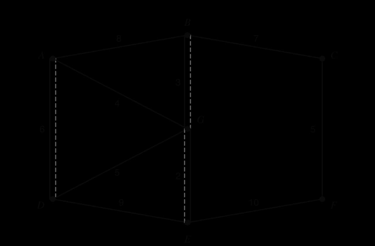
A farming cooperative plans irrigation pipes between seven farms A to G. The possible pipe routes and their lengths in kilometres are shown in the weighted graph.

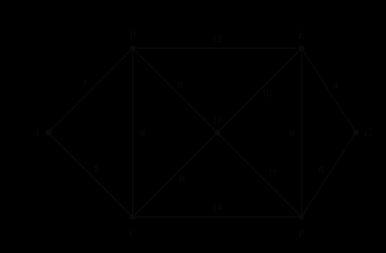
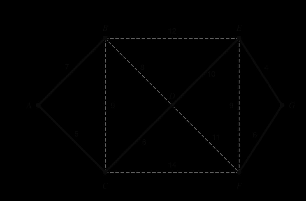
The resulting tree, drawn on the original graph, shows that the cheapest edge between the left half {A, B, C, D} and the right half {E, F, G} is DE, at 10 km; every cheaper edge would have closed a cycle inside one half.

Prim's algorithm

Prim's algorithm grows a single tree outwards from a starting vertex, so the chosen edges are connected at every stage.

1. Choose a starting vertex (often specified in advance).

2. Among all edges that join a vertex in the tree to a vertex not in the tree, choose the one of least weight, and add it and its new vertex to the tree.

3. Repeat step 2 until all $n$ vertices are in the tree.

Prim's algorithm never needs a cycle check: every edge it adds brings in a new vertex, so a cycle can never form. The key point is that the candidate edges come from every vertex in the tree so far, not only from the vertex added last.

Prim's algorithm on a table

When a graph is given as a weighted adjacency table, Prim's algorithm can be carried out on the table itself, without drawing the graph. This matrix method is quick and leaves a clear record of the order of selection. The table gives the lengths, in km, of possible cycle paths between six villages P to U; a blank means no direct path is possible.

In the table, the column of a vertex lists all the edges from that vertex. Numbering a column marks its vertex as "in the tree"; crossing out a row marks that vertex as no longer available as a new vertex.

1. Choose the starting vertex. Cross out its row and write 1 above its column.

2. Look down every numbered column for the smallest entry that has not been crossed out. Circle it.

3. The row of the circled entry gives the new vertex. Cross out that row and write the next number above that vertex's column.

4. Repeat steps 2 and 3 until every row is crossed out. The circled entries are the edges of the minimum spanning tree, and their sum is its weight.

Crossing out rows is what prevents cycles: once a vertex is in the tree, no entry in its row can be chosen, so no edge can lead back into the tree.

The weights in the matrix method are not chosen in increasing order (10 before 8 before 7). That is normal for Prim's algorithm: QS only became available once Q had joined the tree.

Comparing the two algorithms

Both algorithms always find a minimum spanning tree, and both give the same total weight. When all weights are different, there is only one minimum spanning tree, so they also give the same edges. Kruskal's algorithm suits a graph that is drawn with few edges; Prim's matrix method suits a graph given as a table, especially a complete one where listing every edge in order would be slow.

The Chinese postman problem

A postal worker, a street sweeper or a gritting lorry must travel along every edge of a network at least once and return to the start, covering as little distance as possible. If the graph is Eulerian, an Eulerian circuit does the job with no repeats. Otherwise some edges must be travelled twice, and the problem is to choose the cheapest repeats.

Why repeating shortest paths works

A closed route along every edge is an Eulerian circuit of a graph in which the repeated edges are drawn twice. For that larger graph to have an Eulerian circuit, every vertex must have even degree. Repeating an edge adds 1 to the degree of each of its ends, so repeating every edge along a route from one odd vertex to another makes those two vertices even and leaves the vertices in between even (each gains 2).

The cheapest way to make two odd vertices even is therefore to repeat the shortest path between them. With more odd vertices, they must be split into pairs, and the shortest path for each pair repeated.

The shortest path between two vertices is not always the direct edge. In the junction graph, the direct road from P to Q is 9 km, but P → T → Q is only $3 + 4 = 7$ km.

With four odd vertices A, B, C and D there are exactly three ways to split them into two pairs: AB with CD, AC with BD, and AD with BC. Each must be checked, because the best one cannot be predicted.

The algorithm

1. List the odd vertices.

2. No odd vertices: the graph is Eulerian. The shortest route is the total weight of all edges.

3. Two odd vertices: find the shortest path between them. Shortest route = total weight + weight of that shortest path.

4. Four odd vertices: for each of the three pairings, find the shortest path for each pair and add the two weights. Choose the pairing with the smallest sum. Shortest route = total weight + that smallest sum.

5. State which edges are repeated (those on the chosen shortest paths). If an actual route is needed, write down an Eulerian circuit of the graph with those edges doubled.

Four odd vertices

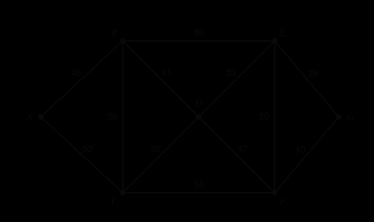
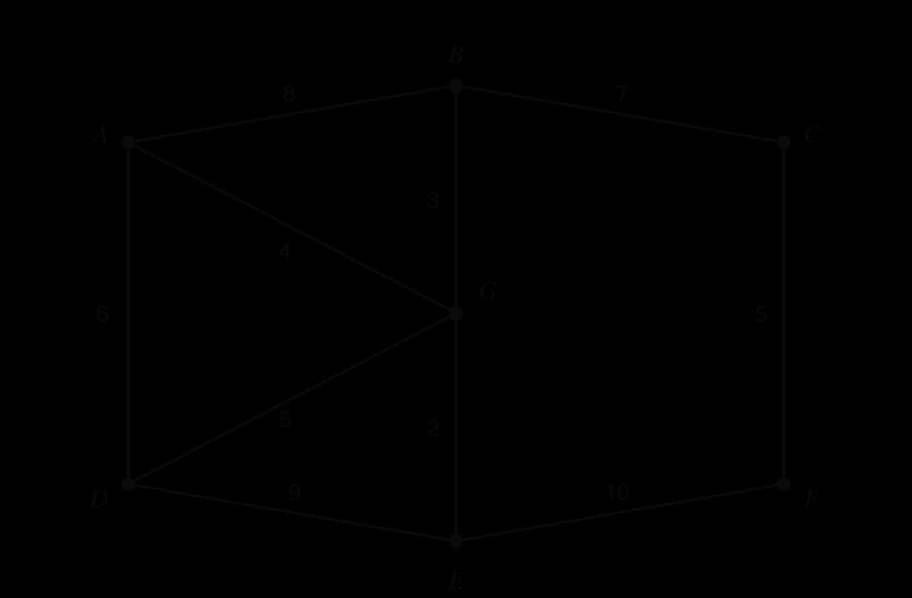
A park ranger inspects every path in a nature park, starting and finishing at the visitor centre A. The walking times in minutes are shown in the graph; the total of all the times is 59 minutes.

Starting and finishing at different vertices

Sometimes the route need not be closed: a sweeper may be dropped at one junction and collected at another. An open route along every edge is an Eulerian trail of the graph with its repeats, so exactly two vertices may stay odd, and those two become the start and the finish.

• Two odd vertices: start at one and finish at the other. No edge needs to be repeated, and the length is just the total weight.

• Four odd vertices: only one pair needs a repeated shortest path. Choose the pair with the smallest single shortest path, repeat it, and start and finish at the other two odd vertices.

The travelling salesman problem

The travelling salesman problem covers every vertex of a graph rather than every edge. A sales representative, a delivery driver or a drill moving across a circuit board must visit each location once and return to the start, by the shortest possible route.

YouTube

From a practical problem to the classical problem

Real road networks are rarely complete graphs, and the shortest way between two places may pass through a third. In a practical problem a route may pass through a vertex more than once on the way to somewhere else. The standard method turns this into the classical problem by replacing every weight with the shortest possible distance between the two vertices.

A table of least distances describes a complete graph, so a Hamiltonian cycle always exists in it. Each entry also satisfies the triangle inequality: going from X to Z directly is never longer than going via Y. A least-distance entry that does not use the direct edge is simply a reminder that the real route passes through other places.

A tourist staying at a hotel A plans a day visiting four sights B, C, D and E and returning to the hotel. The walking times between them, in minutes, are shown in the graph.

Why exact solutions are hard

A complete graph on $n$ vertices has $\frac{(n - 1)!}{2}$ distinct Hamiltonian cycles, so checking them all is possible only for very small $n$.

No method is known that solves every travelling salesman problem quickly as the number of vertices grows. Computer scientists describe problems of this difficulty with a technical term.

Large instances are still solved with clever methods and a great deal of computing. In 2004 an optimal tour through all 24,978 towns in Sweden, about 72,500 km long, was found and proved optimal; in 2006 an 85,900-point instance from a microchip layout was solved. For everyday problems it is usually enough to know that the best route lies between two numbers: an upper bound, which the optimal route cannot exceed, and a lower bound, which it cannot be shorter than.

These bounds have nothing to do with the upper and lower bounds of a rounded measurement in subtopic 1.6: here they are limits on an unknown optimal route.

The nearest neighbour algorithm: an upper bound

Any actual Hamiltonian cycle gives an upper bound, because the optimal cycle is at most that long. The nearest neighbour algorithm is a quick, greedy way to build a reasonably short one.

1. Start at the given vertex.

2. Move along the edge of least weight to a vertex that has not been visited.

3. Repeat step 2 until every vertex has been visited.

4. Return to the starting vertex along the edge joining them. Add up all the weights.

The algorithm needs a complete graph (or a table of least distances); on an incomplete graph it can get stuck at a vertex whose neighbours have all been visited. Because it is greedy, the last few steps often have to use long edges, and the final edge back to the start can be very long.

The deleted vertex algorithm: a lower bound

A lower bound comes from a different idea. Take the optimal Hamiltonian cycle and delete one vertex X and its two edges. What is left is a Hamiltonian path through the other vertices, which is a spanning tree of the graph without X. That tree weighs at least as much as the minimum spanning tree of the graph without X, and the two deleted edges weigh at least as much as the two smallest edges at X.

1. Delete a vertex X and all its edges.

2. Find a minimum spanning tree of the remaining graph, by Kruskal's or Prim's algorithm, and its weight.

3. Add the two edges of least weight that joined X to the other vertices.

4. The total is a lower bound.

Deleting different vertices gives different lower bounds. All are valid, so the largest gives the most information. If a lower bound equals the weight of a known Hamiltonian cycle, that cycle is optimal.

Choosing the right algorithm

Route problems in context are recognised by what must be covered.

A minimum spanning tree shows which links to build; it gives no order in which to travel them. The Chinese postman algorithm is exact for up to four odd vertices, while the travelling salesman problem usually ends with bounds.

Case study: a tour of five capitals

A traveller plans a round trip by air between five north-west European capitals: Amsterdam (AMS), Berlin (BER), Brussels (BRU), London (LON) and Paris (PAR). The table gives great-circle ("as the crow flies") distances, computed from the coordinates of each city centre and rounded to the nearest kilometre.

Source: great-circle distances calculated with the haversine formula (Earth radius 6371 km) from Wikipedia city-centre coordinates, 2026.

Great-circle distances satisfy the triangle inequality, so the table is already a table of least distances for a complete graph $K_5$. It has only $\frac{4!}{2} = 12$ distinct Hamiltonian cycles, so the bounds can be compared with the true optimum.

Upper bounds. The nearest neighbour algorithm from each city gives a different cycle.

The best upper bound is 2291 km. Starting in London gives 2734 km, which is the longest of all 12 possible cycles: after the greedy choices, the route is left in the west and needs two long legs to and from Berlin.

Lower bounds. Deleting each city in turn gives five lower bounds.

Deleting Berlin gives the best (largest) lower bound, because Berlin is far from every other city: its two shortest edges, 577 km and 651 km, are much longer than the shortest edges at any other city. The traveller's optimal round trip therefore lies in the interval

Checking all 12 cycles shows the optimum is AMS → LON → PAR → BRU → BER → AMS, at $357 + 344 + 264 + 651 + 577 = 2193$ km. The best nearest neighbour cycle is 98 km (about 4.5%) longer than the optimum, and the best lower bound is about 9.4% below it. Neither bound alone identifies the optimum; with five cities, listing every cycle is quick, but the same check for 20 cities would need about $6.08 \times 10^{16}$

The model has limitations. Aircraft do not fly exact great-circle routes between city centres, airports are outside the centres, and a traveller cares about time and cost as much as distance. A direct flight may not exist for every pair, in which case the practical problem would need a least-distance table of real connections.

Exam focus

Tree and cycle algorithms appear on HL Papers 1, 2 and 3. Paper 1 usually asks for one algorithm in 4–8 marks (a minimum spanning tree, a Chinese postman route or a pair of bounds). Paper 2 and Paper 3 combine several in a long context, often with a graph given as a table, an unknown weight $x$ to find, or links to adjacency matrices (subtopic 3.15), the cosine rule or probability. Questions use use (a named algorithm), find, write down, state, with a reason, determine, explain, justify and show clearly the order.

• Show the order of edges for Kruskal's, Prim's and nearest neighbour algorithms, and show the sum of the weights for every total.

• Give the degree reason for Eulerian questions.

• For the Chinese postman problem, show the odd vertices, all three pairings and the repeated edges.

• For bounds, say which is upper and which is lower, and choose the smallest upper bound and the largest lower bound.

• No formulas for these algorithms appear in the formula booklet: the steps, Euler's conditions, $n - 1$ edges in a spanning tree and $\frac{(n-1)!}{2}$

Pairing totals are a common source of lost marks. A pairing total that uses a direct edge when a shorter indirect route exists (here A–E has no direct road at all, and B–F must go through D) is marked wrong, and the error carries into the final total.

Questions with an unknown weight $x$ reward reasoning from the algorithm's rules: for example, if Prim's algorithm chose edge AB first from A, then AB must be the smallest weight at A; if a lower bound is written as $41 + x$, keep $x$ as a letter until the question gives a value.

Practice questions

1. In a graph with vertices J, K, L, M, N, the edges are JK, KL, LM, MN, NJ and KM. Determine whether each route is a trail, path, circuit or cycle: (a) J → K → M → N; (b) K → L → M → K → J; (c) J → K → L → M → N → J. [3]

2. A connected graph has vertices with degrees 2, 4, 3, 2, 3, 6. State, with reasons, whether it has (a) an Eulerian circuit, (b) an Eulerian trail, and where any trail must start and finish. [3]

3. A graph has edges JK 15, JL 9, KL 11, KM 10, LM 13, LN 8, MN 6, MO 8, NO 7. Use Kruskal's algorithm to find a minimum spanning tree, showing the order in which edges are considered, and state its weight. [4]

4. For the graph in question 3, use Prim's algorithm starting at J, listing the edges in the order they are added. [3]

5. A street sweeper must clean every street of a small estate, with lengths in hundreds of metres VW 5, WX 7, XY 4, YV 6 and VX 11, starting and finishing at V. Find the length of the shortest route and state which streets are swept twice. [4]

6. A graph has edges PQ 3, QR 4, RS 5, SP 6, PT 2, TR 7, QT 8. (a) Find the shortest route that travels every edge and returns to its start. (b) Find the shortest route if it may start and finish at different vertices, stating where it starts and finishes. [7]

7. The complete graph on A, B, C, D, E has weights AB 14, AC 9, AD 17, AE 11, BC 12, BD 8, BE 16, CD 13, CE 10, DE 15. (a) Use the nearest neighbour algorithm from A to find an upper bound. (b) Use the deleted vertex algorithm, deleting A, to find a lower bound. (c) Find a second lower bound by deleting B and write down the best interval for the optimal cycle. [9]

8. Find the number of distinct Hamiltonian cycles in $K_7$

Summary

• A walk may repeat anything; a trail repeats no edge; a path repeats no vertex; a circuit is a closed trail; a cycle is a closed path.

• In a connected graph, an Eulerian circuit exists exactly when every vertex is even, and an Eulerian trail (not closed) exactly when there are two odd vertices, which are its ends.

• A Hamiltonian path or cycle visits every vertex exactly once; there is no simple test, and $K_n$ has $\frac{(n-1)!}{2}$

Self-check

• To do:

  I can classify a route as a walk, trail, path, circuit or cycle by checking repeated edges and vertices.

• To do:

  I can explain, using arrivals and departures, why an Eulerian circuit needs every vertex to be even.

• To do:

  I can state whether a graph has an Eulerian trail or circuit, with the degree reason, and write one down.

• To do:

  I can explain why a particular graph has no Hamiltonian cycle without using odd vertices.

• To do:

  I can find the number of Hamiltonian cycles in a complete graph.

• To do:

  I can use Kruskal's algorithm, rejecting edges that make cycles and stopping at $n - 1$ edges.

• To do:

  I can use Prim's algorithm from a given vertex, choosing from every vertex in the tree.

• To do:

  I can carry out Prim's matrix method on a weighted adjacency table.

• To do:

  I can find shortest paths by inspection, including indirect routes shorter than a direct edge.