1.8 Equations and systems using technology

Introduction

Many real problems involve several unknown quantities at once: the prices of three items from three till receipts, the currents in the branches of an electric circuit, or the three numbers that fix a curve passing through measured data. Each piece of information becomes an equation, and the unknowns are the values that make every equation true together. Other problems lead to a single equation with powers of the unknown, such as the dimensions of a container of given volume or the times when a cubic profit model equals zero.

A graphic display calculator (GDC) solves both kinds of equation in seconds, so the mathematical work moves to the two ends of the problem: translating the situation into correct equations, and translating the calculator's numbers back into a sensible answer. Both steps need a clear understanding of what a system of equations is, how many solutions a polynomial equation can have, and what each solution means.

Equations, unknowns and solutions

An equation states that two expressions have the same value. When the expressions contain a letter standing for an unknown number, the equation is true for some values of the letter and false for others. Solving the equation means finding every value that makes it true.

The simplest equations involve each unknown only to the first power, multiplied by a number. The equation $3x + 2y = 18$ is of this kind, and so is $0.5a - 4b + c = 7$. Each unknown appears on its own, never squared, never multiplied by another unknown, never inside a root or a denominator.

The name comes from the graph. An equation such as $3x + 2y = 18$ can be rearranged to $y = 9 - 1.5x$, whose graph is a straight line. Every point $(x, y)$ on that line is a pair of values that satisfies the equation, so a single linear equation in two unknowns has infinitely many solutions: $(0, 9)$, $(2, 6)$, $(4, 3)$, $(6, 0)$, $(1, 7.5)$ and so on.

To pin down the values of two unknowns, one equation is not enough. A second, different piece of information gives a second line, and the values that satisfy both equations are the coordinates of the point where the two lines meet.

Systems of linear equations

A solution of a system is a set of values, one for each unknown, that makes every equation true. For the system $3x + 2y = 18$, $x - y = 1$, the values $x = 4$ and $y = 3$ work in both: $3(4) + 2(3) = 18$ and $4 - 3 = 1$. The pair $x = 2$, $y = 6$ satisfies the first equation but not the second, so it is not a solution of the system.

The graphical picture in two unknowns

Each linear equation in two unknowns is a straight line, so a system of two such equations is a pair of lines. A point lies on both lines only where they cross, and the coordinates of that point of intersection are the solution of the system.

Two straight lines in a plane can meet in three ways, and these give the three possible outcomes for any linear system.

The first case is the one that answers a question, because it fixes the value of every unknown.

A system has no solution when its equations contradict each other, and infinitely many when one equation repeats information the others already give. In a well-posed problem from a real context, both situations signal an error: either a piece of information has been translated wrongly, or two equations say the same thing in different words.

Why a system can be solved: elimination

Solving a system by hand shows what the GDC is doing. The idea is to combine the equations so that one unknown disappears, leaving a simpler equation with fewer unknowns. For the system $3x + 2y = 18$ and $x - y = 1$, doubling the second equation makes the $y$-terms opposites, and adding the two equations removes $y$.

The same idea works for three unknowns: two pairs of equations are combined to remove the same unknown, which leaves two equations in two unknowns, and then the step is repeated. The process is routine but long, and each step is a chance for an arithmetic slip. A GDC carries out exactly this kind of elimination internally, in a fraction of a second and without slips, which is why technology is the standard method for systems of three equations.

Three equations in three unknowns

Three unknowns need three independent pieces of information. An equation such as $2x + y - z = -1$ has infinitely many solutions on its own, and two such equations still leave one unknown free. Only a third equation, carrying information the first two do not, fixes all three values.

There is a geometric picture here too. A linear equation in three unknowns describes a flat plane in three-dimensional space, and the solution of a system of three such equations is the single point where all three planes meet. Three planes can also fail to meet at a single point (two of them parallel, or all three sharing a line), which corresponds to no solution or infinitely many solutions, exactly as for lines.

Solving a system with the GDC

Every GDC has a simultaneous equation solver. It needs each equation in standard arrangement: all the unknowns on the left, in the same order in every equation, with the constant on the right. The calculator then takes the numbers only, so the coefficients must be entered in the right columns.

1. Rearrange each equation into the form $ax + by + cz = d$, with the unknowns in the same order.

2. Write a coefficient of 0 for any unknown missing from an equation, and 1 or −1 where no number is written.

3. Open the solver and choose the number of equations and unknowns: on a TI-84 Plus CE, APPS → PlySmlt2 → SIMULTANEOUS EQN SOLVER; on a Casio fx-CG50, MENU → Equation → SIMUL.

4. Enter the coefficients row by row, one equation per row, with the right-hand constant in the last column.

5. Solve, and copy each value with its label, keeping full accuracy for any later calculation.

The arrangement for the system $2x + y - z = -1$, $x - 3y + 2z = 13$, $3x + z = 10$ is shown in the table, exactly as the coefficients go into the solver.

The zero in the third row stands for the missing $y$-term. Leaving it out would push the 1 into the $y$-column and give the calculator a different system with a different answer.

When a solver cannot find a unique solution, it reports an error or a message such as "no solution" or "infinitely many solutions". In a problem built from a real context that message almost always means an equation has been set up or entered wrongly, so each equation is rechecked against the information and re-entered before the solver is used again.

Forming a system from a context

In a real problem, writing the equations takes most of the work. A reliable approach has four parts: define the unknowns, turn each piece of information into one equation, check that there are as many independent equations as unknowns, and solve.

Defining the variables

Each unknown gets a letter and a precise meaning, including its units. "Let $a$ be the number of adult tickets sold" is precise. "Let $a$ be adults" is too vague, because it does not say whether $a$ counts tickets, people or money. Units must also be consistent across all the equations: if one price is in dollars and another in cents, one of them is converted before any equation is written.

Turning statements into equations

Most statements in word problems fall into a few patterns, and each pattern has a standard translation.

The ratio statement is the one most often reversed. In "three times as many adult tickets as senior tickets", the adult number is the larger one, so the 3 multiplies the smaller number, $s$, to make the two sides equal. A test with small numbers confirms the direction: if 10 senior tickets were sold, there were 30 adult tickets, and $a = 3s$ gives $30 = 3 \times 10$, while $3a = s$ would give $90 = 10$.

Checking the solution makes sense

A solver gives numbers without any check of whether they fit the situation, so the solution is checked against the context. Numbers of people or objects must be non-negative whole numbers; prices and masses must be positive; a value far larger than the totals in the question signals an error. A non-integer number of tickets, such as $c = 187.4$, means the system has been formed wrongly, because a correct model of whole tickets cannot produce a fraction of a ticket.

Some quantities can legitimately come out negative, and then the sign carries meaning. A negative current means the current flows the opposite way to the direction assumed; a negative temperature on the Celsius scale is below freezing; a negative balance is a debt. Interpreting the sign is part of the answer.

Kirchhoff's laws in an electric circuit

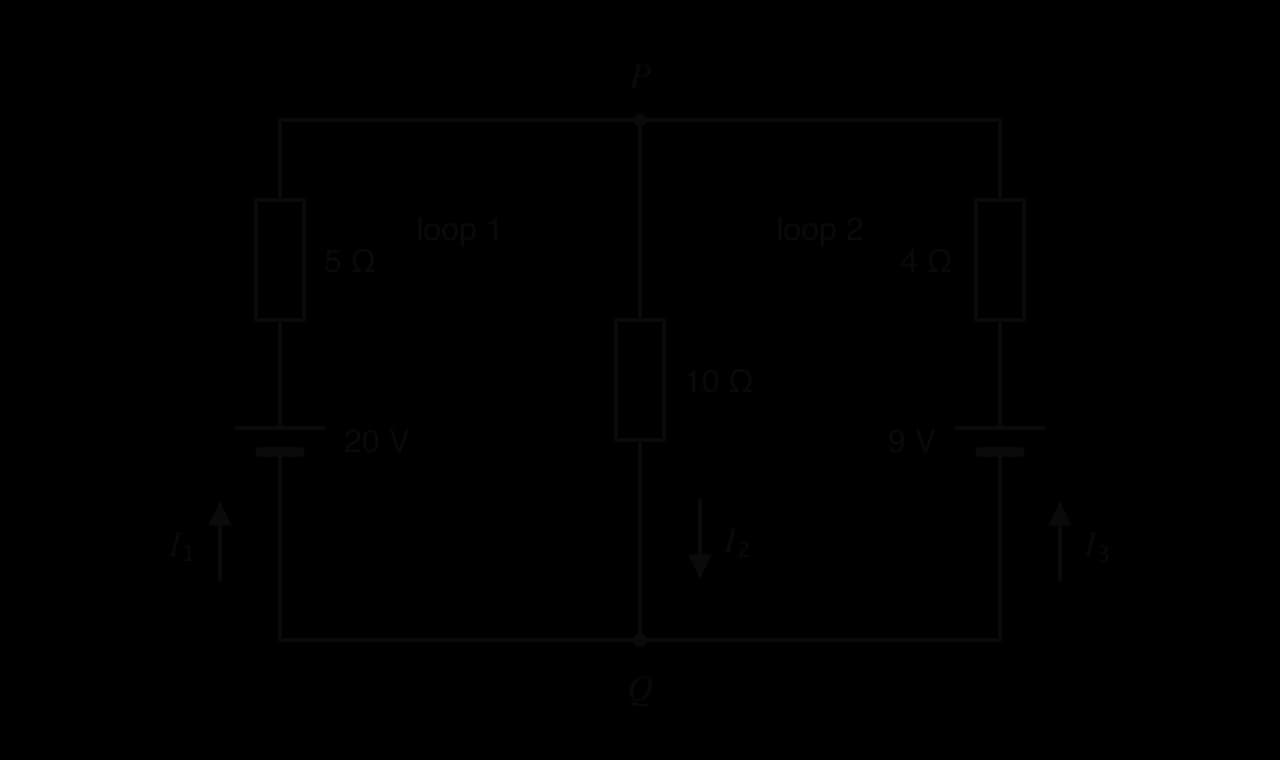
Electrical engineers find the currents in a circuit by solving a linear system. Two physical laws, named after Gustav Kirchhoff, supply the equations. The junction rule says that the total current flowing into a junction equals the total current flowing out, because electric charge is not created or lost. The loop rule says that around any closed loop, the voltages supplied by the cells equal the voltage drops across the resistors, where the drop across a resistance $R$ carrying current $I$ is $IR$.

The circuit in the diagram has three branches meeting at the junctions $P$ and $Q$, so it has three unknown currents. The direction of each current is a guess drawn as an arrow before any calculation; the solution confirms or corrects each guess.

Finding a model's parameters from points

A model such as $y = ax^2 + bx + c$ has a fixed shape (a parabola) but unknown numbers $a$, $b$ and $c$, its parameters. Each point the curve must pass through supplies one equation. Because a point $(x_1, y_1)$ lies on the graph exactly when $y_1 = a x_1^2 + b x_1 + c$, substituting the coordinates gives a linear equation in $a$, $b$ and $c$: the powers of $x$ become numbers, and the unknowns appear only to the first power.

Three points give three linear equations, which is exactly the number needed for three unknown parameters. A cubic model $y = ax^3 + bx^2 + cx + d$ has four parameters and needs four points.

Writing each equation in simplified form

Each substituted equation should be simplified before it is used: powers evaluated, like terms collected, and the equation arranged with the parameters on the left. The simplified form $25a + 5b + c = 38$ can be entered in a solver directly. The unsimplified form $38 = a(5)^2 + b(5) + c$ is correct but unfinished, and it leads to mistakes such as entering 5 instead of 25 in the solver.

When one of the points has $x = 0$, substitution gives the constant directly: at $x = 0$ every term with $x$ vanishes, so $y = c$ for a quadratic and $y = d$ for a cubic. That point therefore removes one unknown immediately and reduces the size of the system.

The final part of the fountain example is a polynomial equation, and the same pattern appears in most modelling questions: a system finds the parameters, and then a polynomial equation answers a question about the model. The rest of the subtopic deals with polynomial equations in full.

Polynomials

The functions $h(x) = -0.52x^2 + 2.24x + 0.56$ and $x^3 - 2x^2 - 5x + 7$ are built in the same way: a sum of terms, each a number times a whole-number power of $x$. Expressions of this kind are the most widely used family of functions in modelling, because they are easy to evaluate and can bend in as many places as a situation needs.

Each term has two parts: a number, and a power of the variable. The numbers carry the information that distinguishes one polynomial from another of the same shape.

The coefficient of a power that does not appear is 0, and a term written without a number, such as $-x$, has coefficient −1. Both facts matter whenever a polynomial is entered into a GDC, which needs every coefficient in order.

The highest power present sets the overall shape of the graph, the number of times it can turn, and the number of solutions an equation can have.

The term with the highest power is the leading term, and its coefficient the leading coefficient. For $0.5x^5 - 3x^2 + 4$, the leading term is $0.5x^5$, the leading coefficient is 0.5 and the constant term is 4. A polynomial does not have to be written in descending order of powers: $4 - 3x^2 + 0.5x^5$ is the same polynomial, and its degree is still 5.

The condition $a \ne 0$ in each general form keeps the degree correct: if the leading coefficient were 0, the term would vanish and the polynomial would have a lower degree.

Polynomial equations

Setting a polynomial equal to zero, or to any number, gives an equation whose unknown appears in powers. Every such equation can be rearranged so that one side is zero.

Polynomial equations of degree 1 are linear equations. The next two degrees have their own names, because they occur so often in models of area, projectile motion, volume and profit.

A quadratic equation arises whenever two lengths are multiplied (an area), whenever a quantity falls under constant acceleration (the height of a thrown ball), and whenever a quadratic model is set equal to a value, as in the fountain example. A cubic equation arises in the same way from a volume, a product of three lengths, or from a cubic model.

Roots and zeros

Two words describe the solutions of a polynomial equation. "Root" describes them as solutions of the equation, and "zero" describes the same numbers as inputs of the function and points on its graph.

A function $p$ gives an output for each input. The inputs that give an output of zero are the places where the graph of $y = p(x)$ meets the $x$-axis.

"Roots of an equation" and "zeros of a function" therefore name the same numbers, and both appear in questions: "solve $p(x) = 0$", "find the roots of the equation", "find the zeros of $p$" and "find the $x$-intercepts of the graph" all ask for the same values, though an intercept is given as a point, such as $(2, 0)$, rather than a number.

The link with factors explains why. If a polynomial factorises as $p(x) = (x - 2)(x - 3)$, then $p(2) = 0 \times (-1) = 0$, because one factor is zero. In general, $x = r$ is a root of $p(x) = 0$ exactly when $(x - r)$ is a factor of $p(x)$. A cubic with roots $-2$, 1 and 4 has the form $p(x) = a(x + 2)(x - 1)(x - 4)$ for some non-zero constant $a$.

How many roots a polynomial equation can have

The degree limits the number of roots. A polynomial of degree $n$ can be written as a product of at most $n$ linear factors, and each root needs its own factor $(x - r)$. A polynomial of degree $n$ therefore has at most $n$ real roots. A graph gives the same conclusion: a quadratic turns once, so its graph can cross a horizontal axis at most twice; a cubic turns at most twice, so it can cross at most three times.

A polynomial of odd degree always has at least one real root. For large positive $x$ its leading term dominates and its value has one sign; for large negative $x$ it has the opposite sign, so the graph must cross the $x$-axis somewhere in between. A polynomial of even degree can stay entirely above or below the axis and have no real roots at all.

Repeated roots

Some polynomials contain the same factor more than once. The cubic $x^3 - 3x + 2$ factorises as $(x - 1)^2(x + 2) = (x - 1)(x - 1)(x + 2)$, so the equation $x^3 - 3x + 2 = 0$ has roots 1, 1 and −2. The value 1 is counted twice.

The graph shows a repeated root clearly. Near a single root the polynomial changes sign, so the graph crosses the axis. Near a double root the squared factor $(x - 1)^2$ is never negative, so the polynomial does not change sign: the graph comes down to touch the axis and turns back, with the axis as a tangent at that point.

A GDC solving $x^3 - 3x + 2 = 0$ lists 1 twice (or two values such as 0.99999998 and 1.00000002, because the calculator works numerically). Both describe the same double root, and the answer is written as $x = 1$ (repeated) and $x = -2$. On a graph, a double root can be found with the GDC's minimum or maximum tool when the zero tool struggles, because the point where the graph touches the axis is also a turning point.

Roots that are not real

Some polynomial equations have fewer real roots than their degree. The equation $x^2 + 1 = 0$ needs $x^2 = -1$, and the square of every real number is zero or positive, so no real number works. The graph of $y = x^2 + 1$ lies entirely above the $x$-axis, which shows the same fact.

Many GDC root finders still report such roots, in a form such as $-4.70 + 5.84\mathrm{i}$. These are non-real solutions: the number $\mathrm{i}$ is not on the real number line. In real-world models such as these, every quantity is a real number, so non-real roots are recorded as "no real root" and discarded. A cubic always has at least one real root, so a cubic root finder that shows one real value and two non-real ones means the graph crosses the $x$-axis exactly once.

Solving polynomial equations with the GDC

A by-hand method exists for some polynomial equations: when a polynomial factorises neatly, setting each factor equal to zero gives the roots. The equation $x^2 - 5x + 6 = 0$ becomes $(x - 2)(x - 3) = 0$, so $x = 2$ or $x = 3$. Most equations from real contexts do not factorise with whole numbers, however, and their roots are irrational decimals. The GDC finds them to many digits in two different ways: the polynomial root finder and the graph.

Method 1: the polynomial root finder

The root finder takes the coefficients of a polynomial, in descending order of powers, and returns every root, real and non-real. It works only for an equation of the form $p(x) = 0$, so rearranging comes first.

1. Rearrange the equation so that one side is 0: $a_n x^n + \dots + a_1 x + a_0 = 0$.

2. Write down the degree $n$ and list all $n + 1$ coefficients in descending order of powers, using 0 for each missing power.

3. Open the root finder and choose the degree: on a TI-84 Plus CE, APPS → PlySmlt2 → POLYNOMIAL ROOT FINDER; on a Casio fx-CG50, MENU → Equation → POLY.

4. Enter the coefficients and solve.

5. Copy the real roots, ignore any non-real ones, and round only the final answers (3 significant figures unless a question asks otherwise).

For the quartic $x^4 + x^3 - 4x - 6 = 0$, the coefficients are 1, 1, 0, −4, −6. The 0 holds the place of the missing $x^2$-term. Without it, the four numbers 1, 1, −4, −6 would describe the cubic $x^3 + x^2 - 4x - 6$, a different polynomial with different roots. With the 0 in place, the root finder gives two real roots, $x = 1.68$ and $x = -1.32$, and two non-real roots.

Method 2: the graph

A graph gives the same roots and also shows how many to expect. There are two versions.

• Zeros: rearrange to $p(x) = 0$, graph $y = p(x)$, and use the GDC's zero (or root) tool at each point where the graph meets the $x$-axis (2nd TRACE → zero on a TI-84 Plus CE; SHIFT F5 (G-SOLVE) → ROOT on a Casio fx-CG50).

• Intersection: leave the equation as it is, graph each side as a separate function, $y = x^3 + 7$ and $y = 2x^2 + 5x$, and use the intersection tool. The $x$-coordinates of the points of intersection are the roots.

The graphical method works for any equation, including ones that are not polynomials, and it shows at once whether a root lies outside the window or is repeated. Its weakness is the viewing window: a root off the screen is easily missed. Subtopic 2.4, Key features of graphs, treats the zero and intersection tools in full.

Rejecting roots in context

Solving a polynomial equation uses only its coefficients, not the situation it came from, so some of its roots may not make sense. Lengths and times in a model are usually positive, a model applies only on its domain, and non-real roots never describe a measurable quantity. Each root is checked against the context, and any root that is rejected is rejected with a reason.

Interpreting every root of a model

A model can produce several roots inside its domain, and each one marks a moment when the quantity changes sign. A profit, a balance or a height above a reference level is positive on some intervals and negative on others, and the roots are the boundaries. The question "for how long is the quantity negative?" is answered by adding the lengths of the intervals between roots where the graph lies below the axis, which needs every root.

Case study: The density of water near its maximum

Most liquids become steadily less dense as they warm, because their molecules move further apart. Pure water behaves differently between 0 °C and about 4 °C: its density rises as it warms, reaches a maximum at about 3.98 °C, and only then starts to fall. A straight line cannot describe a quantity that rises and then falls, but a quadratic with a negative leading coefficient can, so the density of water near its maximum is a natural test of a quadratic model fitted through three measurements. The table gives the measured density of pure water at eleven temperatures from 0 °C to 40 °C.

Source: density of pure water at standard atmospheric pressure, CRC Handbook of Chemistry and Physics (2004) and Lange's Handbook of Chemistry (1999), as tabulated in Wikipedia, "Water (data page)", 2026; converted from g cm⁻³ to kg m⁻³.

Fitting the quadratic

Let $T$ be the temperature in °C and $\rho$ the density in kg m⁻³, with the model

The three readings at 0 °C, 10 °C and 20 °C, $(0, 999.8395)$, $(10, 999.7026)$ and $(20, 998.2071)$, give three linear equations in $a$, $b$ and $c$:

The GDC's simultaneous equation solver, with rows $(0, 0, 1 \mid 999.8395)$, $(100, 10, 1 \mid 999.7026)$ and $(400, 20, 1 \mid 998.2071)$, gives $a = -0.006793$, $b = 0.05424$ and $c = 999.8395$, all exact. The model is

Each parameter has a meaning. The value of $c$ is the density at 0 °C. The positive value of $b$ means the density increases as water warms from 0 °C, which is the unusual behaviour of water. The negative value of $a$ bends the graph downwards, so the increase slows, stops and turns into a decrease, producing a maximum.

This model shows how much the accuracy of the parameters matters. All the densities lie within 2 kg m⁻³ of each other, so the information sits in the last few digits. Rounding the parameters to 3 significant figures turns $c$ into 1000 and gives $\rho(20) = 998.368$ kg m⁻³ instead of the measured 998.2071, an error of 0.16 kg m⁻³, larger than the error of the full-accuracy model at every temperature from 0 °C to 25 °C. The parameters are stored in the GDC and used at full accuracy, and only final answers are rounded.

Using a polynomial equation to locate the maximum

The parabola is symmetric about its vertical axis, so the temperature of maximum density lies halfway between any two temperatures with equal density. Setting the model equal to its value at 0 °C gives a quadratic equation:

The polynomial root finder (coefficients −0.006793, 0.05424, 0) gives $T = 0$ and $T = 7.9846\ldots$. The model predicts that water at about 7.98 °C has the same density as water at 0 °C, and that the maximum lies halfway between, at $T = 3.99$ °C, with $\rho(3.9923\ldots) = 999.948$ kg m⁻³. The GDC's maximum tool on the graph of $\rho$ gives the same point. The measured maximum is 999.972 kg m⁻³ at about 3.98 °C, so the model places the maximum within 0.01 °C of the measured temperature, although none of the three readings used is near 4 °C.

Testing the model

A model built from three points passes through those points exactly, so its quality shows in the temperatures that were not used. The table compares the model with the other eight measurements.

From 0 °C to 22 °C, the range of the three readings used and just beyond it, every prediction is within 0.03 kg m⁻³ of the measurement, an error of less than 0.003%. Beyond 20 °C the errors grow steadily, reaching −1.07 kg m⁻³ at 40 °C, because the real density curve falls less steeply than the parabola at higher temperatures. The graph of the model with all eleven measurements shows the same pattern.

Using the model: when does the density fall to 998 kg m⁻³?

Setting the model equal to 998 gives a quadratic equation:

The polynomial root finder gives $T = 20.93\ldots$ or $T = -12.94\ldots$. The negative root is rejected because pure water at normal pressure freezes at 0 °C, so temperatures below 0 °C lie outside the domain of the model. The model predicts a density of 998 kg m⁻³ at 20.9 °C. The measurements put the true temperature between 20 °C (998.2071) and 22 °C (997.7735), consistent with the prediction.

The same question for 994 kg m⁻³ would need an extrapolation beyond 30 °C, where the testing table shows the model's errors are growing, so the answer would be unreliable. The quadratic is therefore a good model of water between 0 °C and about 22 °C only. Fitting a curve to every measurement at once is a regression problem, taught in subtopic 4.4, Correlation and regression (for straight lines), and for HL students in subtopic 4.13, Non-linear regression. The maximum density near 4 °C has a visible consequence: in a deep freshwater lake in winter, water at about 4 °C sinks to the bottom and stays there while ice forms at the surface.

Exam focus

Equations and systems solved with technology rarely appear as a whole question on their own. They are usually one or two parts of a longer modelling question on Paper 1 or Paper 2, often filed under functions or modelling: forming the equations for a model's parameters, solving them, and then solving a polynomial equation to answer a question about the model. Typical parts are worth 2–6 marks.

• Write down the equations: an A1 is usually awarded for each correct, simplified equation, and equivalent forms are accepted. Equations left with unevaluated powers or uncollected terms risk losing marks.

• Find or solve: no particular method is required, and the system always has a unique solution. Solving three equations by hand wastes time; the GDC is expected.

• Show that an equation holds: substitute the point and simplify forwards to the given result.

• Hence or hence or otherwise: use the equations from the previous part (a correct alternative method is credited with "otherwise").

• Interpret: give the meaning of a root or a parameter in context, with units.

Marks for solutions are often split, for example one mark for all three correct values and one for labelling which value belongs to which variable. Roots are given to 3 significant figures unless the question asks otherwise.

The commonest question shape builds a model from points, as in this question. Another gives information in words (numbers of items and their total cost, or a mixture with ratio conditions) and asks for three equations and their solution. A third gives a polynomial model directly and asks when it reaches a given value, which is a polynomial equation after rearranging.

Questions on polynomial equations in context reward interpretation more than calculation. After finding the roots, decide which ones lie in the domain, reject the others with a reason, and use all the remaining roots when the question concerns intervals of time or ranges of values.

Practice questions

1. For the polynomial $p(x) = 6 - 2x^3 + 0.8x^4$, write down (a) its degree, (b) the coefficient of $x^3$, (c) the coefficient of $x^2$, (d) its constant term. [4]

2. Solve the system $4x - y = 11$, $3x + 2y = 22$. [2]

3. Solve the system $2x - 3y + z = 6.4$, $x + 4y - 2z = -4.5$

4. At a café, 2 coffees, 1 tea and 2 slices of cake cost $19.50; 3 coffees, 2 teas and 1 slice of cake cost $21.70; and 1 coffee, 1 tea and 3 slices of cake cost $20.20. (a) Write down three equations to represent this information, defining your variables. [3] (b) Find the price of each item. [2]

5. Find the roots of $x^3 - 4x^2 - 7x + 10 = 0$, and write down the coordinates of the points where the graph of $y = x^3 - 4x^2 - 7x + 10$

6. Solve $0.2x^4 + x + 4 = 3x^2$. [3]

7. The height, $h$ metres, of a ball $t$ seconds after it is thrown is modelled by $h(t) = at^2 + bt + c$. The ball is at a height of 18.2 m after 1 second, 25.2 m after 2 seconds and 9.2 m after 4 seconds. (a)

8. Explain why a cubic equation must have at least one real root, and state the maximum number of real roots of a polynomial equation of degree 6. [3]

9. (a) Solve $x^3 - 6x^2 + 9x = 0$. [2] (b) Describe the graph of $y = x^3 - 6x^2 + 9x$

10. A rectangular tank has width $x$ m, length $(x + 2)$ m and height $(x - 0.5)$ m. Its volume is 12 m³. (a) Show that $x^3 + 1.5x^2 - x - 12 = 0$

Summary

• A linear equation has every unknown to the power 1; a system of linear equations is a set of them to be satisfied together, and its unique solution is the one set of values that works in every equation.

• Two linear equations in two unknowns are two lines: one crossing point gives a unique solution, parallel lines give none, the same line gives infinitely many.

• To solve with the GDC: rearrange each equation to $ax + by + cz = d$, use 0 for missing unknowns, enter the coefficients row by row, and label each value in the answer.

• From a context, define each variable with units, turn each statement into one equation (test ratio statements with small numbers), and check the solution makes sense.

• Substituting points into $y = ax^2 + bx + c$ or $y = ax^3 + bx^2 + cx + d$ gives linear equations in the parameters; a point with $x = 0$ gives the constant term directly.

• A polynomial of degree $n$ has at most $n$ real roots; odd degrees always have at least one.

• Roots of $p(x) = 0$, zeros of $p$ and $x$-intercepts of $y = p(x)$ are the same numbers; a repeated root is where the graph touches the axis without crossing.

• To solve a polynomial equation, rearrange to $p(x) = 0$ and use the root finder (coefficients in descending order, zeros for missing powers) or the graph's zero or intersection tool.

• Discard non-real roots, reject roots outside the domain with a reason, and use every remaining root when interpreting intervals in context.

Self-check

• To do:

  I can decide whether an equation is linear.

• To do:

  I can explain what it means for a system to have a unique solution, and describe the other two possibilities using lines.

• To do:

  I can rearrange equations into standard arrangement with 0 for missing unknowns before entering them in a GDC.

• To do:

  I can solve systems of two or three linear equations with the GDC's simultaneous equation solver.

• To do:

  I can define variables precisely and write equations from totals, values and ratio statements without reversing the ratio.

• To do:

  I can check a solution against its context, including the meaning of a negative value.

• To do:

  I can form and simplify equations for the parameters of a quadratic or cubic model from given points.

• To do:

  I can state the degree, coefficients and constant term of a polynomial written in any order.

• To do:

  I can state the maximum number of real roots of a polynomial equation from its degree.

• To do:

  I can explain the link between roots, zeros, factors and $x$-intercepts.

• To do:

  I can recognise a repeated root from a factorised polynomial, a GDC output or a graph.

• To do:

  I can solve a polynomial equation with the root finder, entering every coefficient correctly.

• To do:

  I can solve an equation graphically using the zero or intersection tool.

• To do:

  I can discard non-real roots and reject roots outside a model's domain with a reason.

• To do:

  I can use several roots together to find the total time a model's value is positive or negative.

where $k$ is a constant and distances are measured in metres. The two cables are perpendicular.

1. (a)

   Write down the gradient of $L_1$ in terms of $k$.

   [1]1 mark

   Markscheme (a)

   $-\frac{2}{k}$ A1

   [1 mark]

2. (b)

   Find the value of $k$.

   [2]2 marks

   Markscheme (b)

   $-\frac{2}{k} \times 3 = -1$

3. (c)

   Find the coordinates of the point where the two cables cross.

   [2]2 marks

   Markscheme (c)

   $2x + 6(3x - 4) - 7 = 0$ OR use of GDC to solve the simultaneous equations (M1)

   $(1.55, 0.65)$

4. (d)

   An inspection point is located where $L_2$ crosses the $y$-axis. Find the distance between the inspection point and the point where the two cables cross.

   [2]2 marks

   Markscheme (d)

   inspection point $(0, -4)$

   $\sqrt{(1.55 - 0)^2 + (0.65 - (-4))^2}$

The solver gives

Check in the original equations: $2(2) + (-1) - 4 = -1$ ✓; $2 + 2(4) = 10$ and $3(-1) + 13 = 10$ ✓; $3(2) + 4 = 10$ ✓. All three are satisfied, so the solution is $x = 2$, $y = -1$, $z = 4$.

(b) Loop 1 contains the 20 V cell, the 5 Ω resistor carrying $I_1$ and the 10 Ω resistor carrying $I_2$. The voltage supplied equals the sum of the drops $IR$:

(c) Loop 2 contains the 9 V cell, the 4 Ω resistor carrying $I_3$ and the 10 Ω resistor carrying $I_2$:

(d) With the unknowns in the order $I_1, I_2, I_3$, the coefficient rows are $(1, -1, 1 \mid 0)$, $(5, 10, 0 \mid 20)$ and $(0, 10, 4 \mid 9)$. The GDC's simultaneous equation solver gives

So $I_1 = 1.73\text{ A}$, $I_2 = 1.14\text{ A}$ and $I_3 = -0.591\text{ A}$, correct to 3 significant figures. (The exact values are $\frac{19}{11}$, $\frac{25}{22}$ and $-\frac{13}{22}$.)

The negative value of $I_3$ means the current in the right-hand branch flows downwards, opposite to the arrow drawn: a current of 0.591 A is pushed backwards through the 9 V cell by the stronger 20 V cell. The assumed direction was wrong, but the equations still give the correct size and, through the sign, the correct direction.

Check at the junction: $1.7272\ldots + (-0.5909\ldots) = 1.1363\ldots$ ✓.

(b) Substituting $(1.5, 2.75)$ and $(3, 2.6)$:

(c) The GDC's simultaneous equation solver, with rows $(0.25, 0.5, 1 \mid 1.55)$, $(2.25, 1.5, 1 \mid 2.75)$ and $(9, 3, 1 \mid 2.6)$, gives

The model is $h(x) = -0.52x^2 + 2.24x + 0.56$.

(d) At $x = 0$, $h = c = 0.56$, so the water leaves the nozzle at a height of 0.56 m above the ground.

(e) The water reaches the ground when $h = 0$:

The GDC's polynomial root finder (degree 2, coefficients −0.52, 2.24, 0.56) gives $x = 4.5446\ldots$ or $x = -0.2369\ldots$. The negative value lies behind the nozzle, outside the domain of the model, so it is rejected. The water reaches the ground 4.54 m from the nozzle.

as required.

(b) The GDC's polynomial root finder (coefficients 1, 3, −4, −360) gives one real root and two non-real roots:

The non-real roots are rejected, since a width is a real length. The width is $x = 6.40$ cm, so the length is $6.4036\ldots + 4 = 10.4$ cm and the height is $6.4036\ldots - 1 = 5.40$ cm.

Check: $6.4036\ldots \times 10.4036\ldots \times 5.4036\ldots = 360.0$ cm³ ✓, and all three lengths are positive.

All three roots lie in the domain $0 \le t \le 6$. The constant term gives $B(0) = 3.2 > 0$, and the leading coefficient is negative, so the sign pattern is: positive before the first root, negative between the first and second, positive between the second and third, and negative after the third. A sketch of the graph on $0 \le t \le 6$ confirms it.

The balance is negative for $0.5457\ldots < t < 2.9007\ldots$ and for $5.0534\ldots < t \le 6$. The total time is

The balance is negative for a total of 3.30 years, correct to 3 significant figures.

$512a + 64b + 8c = 4.8$ A1

Note: accept equivalent equations, for example $8a + 4b + 2c - 6 = 6$. Award at most A1A1A0 if the equations still contain $d$ unsubstituted.

[3 marks]

(c) $a = 0.15$, $b = -2.4$, $c = 10.2$ A1A1

Note: award A1 for all three correct values seen, A1 for all three values correctly labelled.

[2 marks]

(d) $0.15t^3 - 2.4t^2 + 10.2t - 6 = 0$ (M1)

$t = 0.698$, $t = 6.55$, $t = 8.75$ $(0.69781\ldots, 6.54778\ldots, 8.75440\ldots)$ A1

[2 marks]

(e) $0.69781\ldots + (8.75440\ldots - 6.54778\ldots)$ (M1)

$= 2.90$ months $(2.90443\ldots)$ A1

Note: award (M1) for recognising that the business is in debt for $0 \le t < 0.698$ and for $6.55 < t < 8.75$. Do not award the A1 for a single root or a single interval.

[2 marks]

(f) $B(10) = 6$ A1

At the end of the 10 months (the end of December) the business has a positive balance of $6,000 (it is no longer in debt). R1

[2 marks]

Total [12 marks]

$k = 6$ A1

Note: Award the method mark for their gradient from part (a) multiplied by $3$ and equated to $-1$, or for equating their gradient to $-\frac{1}{3}$.

[2 marks]

Note: Follow through from their value of $k$.

[2 marks]

$4.90$ (m) $(4.90153\ldots)$ A1

Note: Follow through from part (c).

[2 marks]

[2]2 marks