1.15 Eigenvalues and eigenvectors

Learning objectives

• Determine whether a given vector is an eigenvector of a 2 × 2 matrix, and state its eigenvalue.

• Find the characteristic polynomial of a 2 × 2 matrix and solve the characteristic equation to obtain the eigenvalues.

• Find an eigenvector for each eigenvalue, giving it in a required form such as integer entries.

• Interpret eigenvectors geometrically as directions that a matrix keeps on the same line through the origin.

• Write down a matrix $P$ of eigenvectors and a diagonal matrix $D$ of eigenvalues with $M = PDP^{-1}$, in matching order.

• Use $M^n = PD^nP^{-1}$ to find a general expression for a power of a matrix.

• Determine the long-term behaviour of a system $\boldsymbol{x}_{n+1} = M\boldsymbol{x}_n$ from its eigenvalues, including the long-term state of a two-state Markov chain.

• Interpret eigenvalues and eigenvectors in contexts such as population movement between two towns, predator–prey models and damped motion.

Introduction

Multiplying a vector by a matrix usually changes both its length and its direction. For almost every matrix, though, a few special directions survive: vectors along them come out on the same line through the origin, only stretched, shrunk or reversed. These directions are the eigenvectors of the matrix, and the stretch factors are its eigenvalues. Once they are known, repeated multiplication by the matrix, which is hard to follow directly, becomes repeated multiplication by ordinary numbers.

That is why eigenvalues appear wherever a system changes in steps or over time. The long-run split of a population moving between two towns, whether two interacting species grow or die out, and whether a car's suspension settles after a bump are all decided by the eigenvalues of a 2 × 2 matrix. Search engines, structural engineers and economists use the same idea with much larger matrices.

Eigenvectors and eigenvalues

What a matrix does to a vector

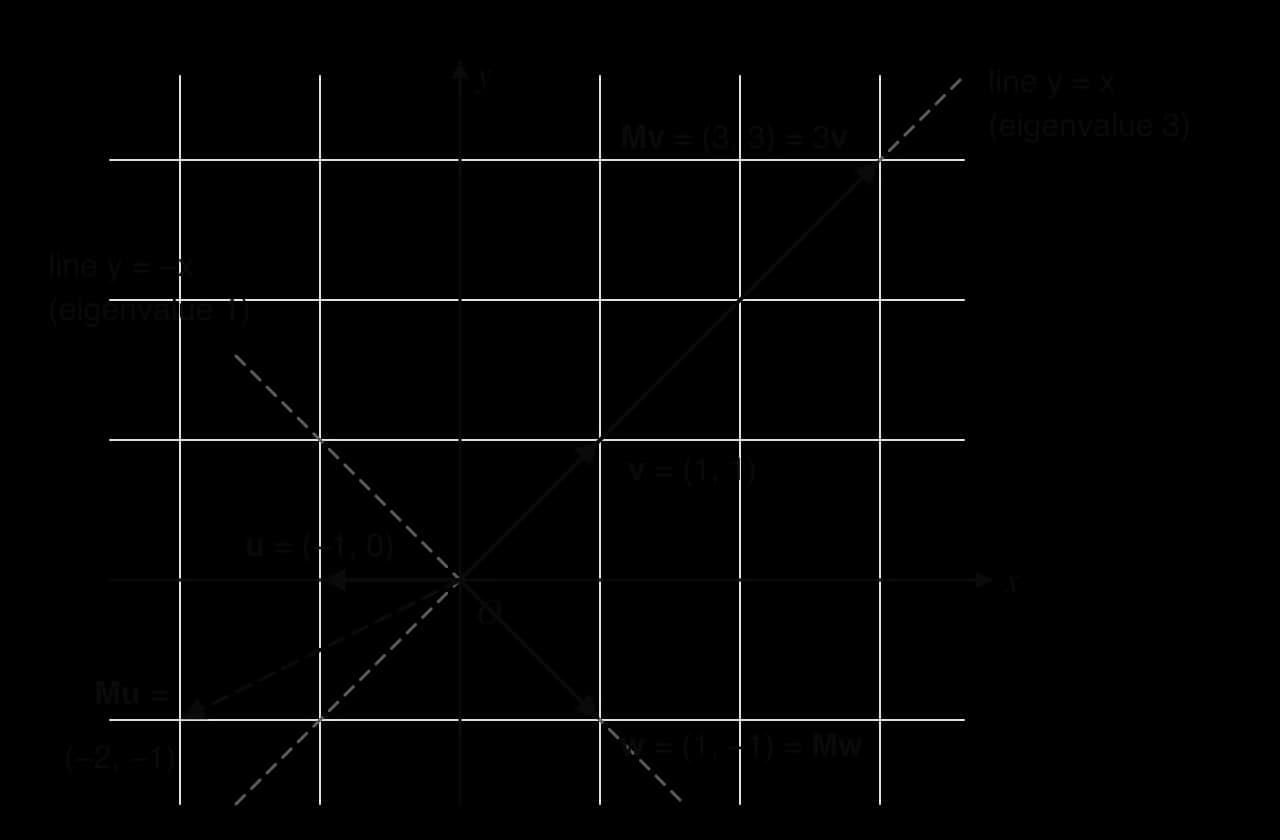
Subtopic 1.14, Matrices, treated a 2 × 2 matrix as a table of numbers. It can also be read as a rule that takes a column vector $\boldsymbol{v}$ and produces a new vector $M\boldsymbol{v}$. Take

Applying $M$ to three vectors gives three quite different results.

The first vector comes out three times as long but pointing the same way. The second comes out unchanged. The third is turned onto a different line: $\begin{pmatrix} -2 \\ -1 \end{pmatrix}$ is not a multiple of $\begin{pmatrix} -1 \\ 0 \end{pmatrix}$

The definitions

The scalar in the equation has its own name. The Greek letter $\lambda$ (lambda) is the standard symbol.

The defining equation is short enough to memorise exactly, and every method for finding eigenvalues and eigenvectors starts from it.

"Eigen" is German for "own" or "characteristic", so the names describe a direction that is characteristic of the matrix and the scale factor that the matrix applies along that direction.

Properties that follow from the definition

Several facts follow directly from $M\boldsymbol{v} = \lambda\boldsymbol{v}$.

• The zero vector is excluded. $M\boldsymbol{0} = \lambda\boldsymbol{0}$ is true for every number $\lambda$, so allowing $\boldsymbol{0}$ would make every number an eigenvalue and the idea would be useless.

• Any non-zero multiple of an eigenvector is also an eigenvector, with the same eigenvalue. If $M\boldsymbol{v} = \lambda\boldsymbol{v}$

A line through the origin made of eigenvectors is mapped onto itself by $M$: every point on it lands somewhere on the same line. In the language of transformations, such a line is an invariant line of the transformation with matrix $M$.

YouTube

The animation in the video shows the same picture as the diagram of $M$: when the whole plane is transformed, most vectors are knocked off their line, while the eigenvectors stay on theirs.

The characteristic polynomial

From Mv = λv to a determinant

Checking given vectors is easy, but the real task is to find the eigenvalues without knowing any eigenvectors. The starting point is to collect everything in $M\boldsymbol{v} = \lambda\boldsymbol{v}$ on one side. Writing $\lambda\boldsymbol{v}$ as $\lambda I\boldsymbol{v}$, where $I$ is the identity matrix

The identity matrix is needed because $M - \lambda$ has no meaning: a number cannot be subtracted from a matrix. $M - \lambda I$ is simply $M$ with $\lambda$ subtracted from each entry on its leading diagonal.

Now suppose $M - \lambda I$ had an inverse. Multiplying both sides on the left by $(M - \lambda I)^{-1}$ would give $\boldsymbol{v} = (M - \lambda I)^{-1}\boldsymbol{0} = \boldsymbol{0}$

Every eigenvalue of $M$ is a solution of this equation, and its left-hand side is a polynomial in $\lambda$.

Setting the polynomial equal to zero gives the equation whose roots are the eigenvalues.

The 2 × 2 formula: trace and determinant

For a general 2 × 2 matrix the determinant can be expanded once and for all.

The constant term $ad - bc$ is $\det M$. The coefficient of $\lambda$ involves the sum of the leading-diagonal entries, which also has a name.

So every 2 × 2 characteristic equation has the same shape:

For a 2 × 2 matrix the characteristic equation is $\lambda^2 - (a + d)\lambda + (ad - bc) = 0$.

A quadratic with roots $\lambda_1$ and $\lambda_2$ factorises as $(\lambda - \lambda_1)(\lambda - \lambda_2) = \lambda^2 - (\lambda_1 + \lambda_2)\lambda + \lambda_1\lambda_2$

Real, repeated or complex eigenvalues

The characteristic equation is a quadratic, so its discriminant decides what kind of eigenvalues the matrix has.

The last row has a clear geometric meaning. The matrix $\begin{pmatrix} 0 & -1 \\ 1 & 0 \end{pmatrix}$ rotates every vector through 90° about the origin, so no non-zero vector stays on its own line, and no real eigenvector can exist. Its eigenvalues are the complex numbers $\pm\mathrm{i}$

Eigenvalues with technology

Every eigenvalue calculation for a 2 × 2 matrix reduces to solving a quadratic, so the GDC's polynomial root finder is the reliable method (on a TI-84 Plus CE: APPS → PlySmlt2 → POLYNOMIAL ROOT FINDER; on a Casio fx-CG50: MENU → Equation → POLY).

1. Work out $\operatorname{tr} M = a + d$ and $\det M = ad - bc$ (the determinant can also come from the matrix menu).

2. Enter the coefficients $1$

Some GDCs also have built-in eigenvalue and eigenvector functions (eigVl( and eigVc( on a TI-Nspire), but not every model does, and the TI-Nspire's Press-to-Test mode blocks them. Whichever tool is used, the characteristic equation itself should be written down: it records how the eigenvalues were found, and without it a wrong eigenvalue cannot be traced back to its cause.

Working backwards: a matrix with an unknown entry

Because $\lambda$ is an eigenvalue exactly when $\det(M - \lambda I) = 0$, a question can give an eigenvalue and ask for an unknown entry. Substituting the known eigenvalue turns the characteristic equation into a linear equation for the unknown. The trace then gives the other eigenvalue at once.

Finding eigenvectors

The method

Once an eigenvalue $\lambda$ is known, its eigenvectors are the non-zero solutions of $(M - \lambda I)\boldsymbol{v} = \boldsymbol{0}$. Writing $\boldsymbol{v} = \begin{pmatrix} x \\ y \end{pmatrix}$

Because $\det(M - \lambda I) = 0$, the two rows of $M - \lambda I$ are multiples of each other, and so the two equations are really the same equation. This is exactly why there are infinitely many solutions (a whole line of them) rather than just $x = y = 0$

1. Write down $M - \lambda I$ with the eigenvalue substituted.

2. Form the equation from one row, for example $px + qy = 0$.

3. Choose a convenient non-zero value for one variable and find the other, or read off the solution $x = q$

If the first row is all zeros, use the second row instead. If both rows are all zeros, every vector is an eigenvector; this happens only for matrices such as $\begin{pmatrix} 3 & 0 \\ 0 & 3 \end{pmatrix}$ that are multiples of $I$.

Choosing a convenient form

Since any non-zero multiple of an eigenvector is an eigenvector, the form can be chosen to suit the question. Integer entries with no common factor are the usual choice, and some questions insist on them. When the matrix has decimal entries, the row equation can be multiplied through to clear the decimals before choosing values.

Special cases

Triangular and diagonal matrices. If $b = 0$ or $c = 0$, the determinant of $M - \lambda I$ is just $(a - \lambda)(d - \lambda)$

A repeated eigenvalue. The matrix $\begin{pmatrix} 3 & 1 \\ 0 & 3 \end{pmatrix}$ has the eigenvalue 3 twice. Then $M - 3I = \begin{pmatrix} 0 & 1 \\ 0 & 0 \end{pmatrix}$

Eigenvectors of familiar transformations

Matrices that represent transformations, taught in subtopic 3.9, Matrix transformations, have eigenvectors that can often be predicted from the geometry, which is a good way to build intuition.

Diagonalisation

Building M = PDP⁻¹

Suppose $M$ has two distinct real eigenvalues $\lambda_1$ and $\lambda_2$, with eigenvectors $\boldsymbol{p}_1$

Multiplying $M$ by $P$ multiplies each column of $P$ by $M$, and each column is an eigenvector. Multiplying $P$ by $D$ on the right multiplies the first column of $P$

When the eigenvalues are different, the two eigenvectors point along different lines, so $\det P \neq 0$ and $P^{-1}$ exists. Multiplying $MP = PD$

The process of rewriting $M$ in this form has its own name.

The order of the factors matters, because matrix multiplication is not commutative: $PDP^{-1}$ is in general different from $P^{-1}DP$. A check that the order is right comes straight from the derivation: $MP = PD$

P and D must match

There is freedom in choosing $P$ and $D$. Either eigenvalue can come first, and each eigenvector can be scaled. What is fixed is the pairing: the eigenvector in column $k$ of $P$ must belong to the eigenvalue in position $k$ of $D$

Why distinct real eigenvalues are needed

Diagonalisation needs two eigenvectors on different lines, so that $P$ is invertible. Two distinct eigenvalues guarantee this: if the eigenvectors were on the same line they would be multiples of each other and would have the same eigenvalue. With a repeated eigenvalue there may be only one eigenvector direction, as for the shear $\begin{pmatrix} 3 & 1 \\ 0 & 3 \end{pmatrix}$

Finding a matrix from its eigenvalues and eigenvectors

The relation $M = PDP^{-1}$ also works in reverse. If the eigenvalues and eigenvectors are known, for example from the geometry of a transformation or from data, the matrix can be rebuilt by multiplying $P$, $D$ and $P^{-1}$

Powers of a matrix

Why diagonal matrices are easy to raise to powers

Raising a general matrix to a power means multiplying it by itself again and again, and the entries of $M^n$ follow no obvious pattern. A diagonal matrix is different: multiplying two diagonal matrices just multiplies the corresponding diagonal entries, so

Diagonalisation transfers this simplicity to $M$. In $M^2 = (PDP^{-1})(PDP^{-1})$

$M^n = PD^nP^{-1}$, where $P$ is a matrix of eigenvectors and $D$

This formula gives $M^n$ as one expression valid for every value of $n$, whereas a GDC evaluates $M^n$ for one chosen value of $n$ at a time. Each entry of $M^n$

Long-term behaviour

The expression $M^n = PD^nP^{-1}$ shows what happens as $n$ becomes large, because the behaviour of $\lambda^n$

For a system that evolves by $\boldsymbol{x}_{n+1} = M\boldsymbol{x}_n$, so that $\boldsymbol{x}_n = M^n\boldsymbol{x}_0$

The numbers $c_1$ and $c_2$ are the entries of $P^{-1}\boldsymbol{x}_0$

• The eigenvalue with the largest size, the dominant eigenvalue, decides the long-run behaviour: its term outgrows the other, so $\boldsymbol{x}_n$ ends up pointing along the dominant eigenvector and grows or shrinks by that factor each step.

• If one eigenvalue is 1 and the other has size less than 1, the second term dies away and $\boldsymbol{x}_n$ settles to the fixed vector $c_1\boldsymbol{p}_1$

YouTube

Applications

Population movement between two towns

Two neighbouring towns, A and B, have populations that change only through people moving between them. Suppose that each year 10% of the people in town A move to town B, and 15% of the people in town B move to town A; everyone else stays. This is a hypothetical but typical model of migration, and the state transition diagram shows the four yearly proportions.

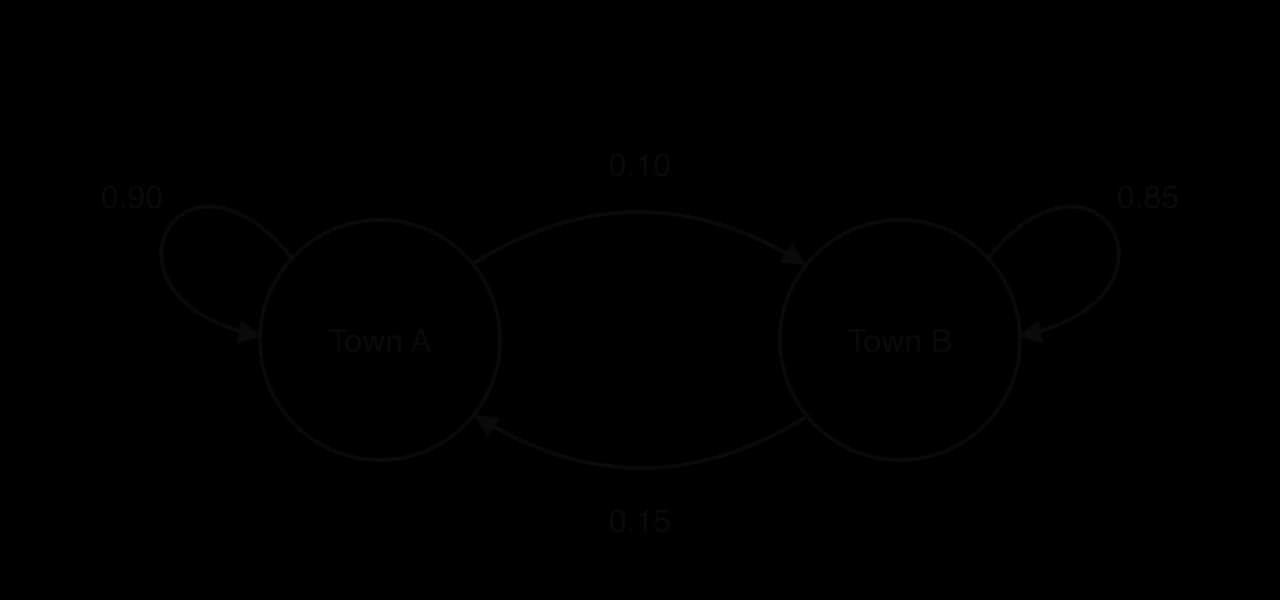
If $a_n$ and $b_n$ are the populations after $n$ years, then next year's population of A is the 90% of A who stay plus the 15% of B who arrive, and similarly for B.

The matrix $T$ is a transition matrix: column 1 gives where the people of A go, and column 2 where the people of B go. Each column adds up to 1 because everyone ends up somewhere. This is a two-state Markov chain, studied in full in subtopic 4.19, Transition matrices and Markov chains.

Eigenvalues. $\operatorname{tr} T = 1.75$ and $\det T = 0.765 - 0.015 = 0.75$, so

Eigenvectors. For $\lambda = 1$, $T - I = \begin{pmatrix} -0.1 & 0.15 \\ 0.1 & -0.15 \end{pmatrix}$

The eigenvalue 1 comes from the column sums. In $T - I$, each column of $T$ has had 1 subtracted from one of its entries, so each column of $T - I$ adds up to 0. The second row is then the negative of the first, the rows are multiples of each other, and $\det(T - I) = 0$

The long-term split of 48,000 to 32,000 is in the ratio $3 : 2$, exactly the ratio of the entries of the eigenvector for $\lambda = 1$. Scaling that eigenvector so that its entries add up to 1 gives the proportions $\begin{pmatrix} 0.6 \\ 0.4 \end{pmatrix}$

The graph of town A's population shows the gap above 48,000 being multiplied by 0.75 each year, so the eigenvalue that is not 1 sets the speed of convergence. A second eigenvalue close to 1 would mean a slow approach to the steady state; one close to 0 would mean the steady state is reached almost at once.

Predator–prey models

A discrete predator–prey model links a predator population $F_n$ and a prey population $R_n$ from one year to the next. In a hypothetical woodland, with $F_n$

Each coefficient has a meaning. Without prey, only half the foxes would survive a year (0.5); rabbits feed the foxes (+0.4); left alone, the rabbits would grow by 20% a year (1.2); and foxes eat rabbits (−0.15). The negative entry is what makes this a predator–prey model rather than a migration model.

The model is linear, so it cannot capture limits such as food supply or space, and it predicts unlimited growth. Over a few years it can still describe how the two populations move together, and the eigenvector gives the balance they settle into. Continuous-time predator–prey models with coupled differential equations are developed in subtopic 5.16, Euler's method, and subtopic 5.17.

Coupled differential equations and damping

Eigenvalues also govern systems that change continuously. A linear system of coupled differential equations $\dot{x} = ax + by$, $\dot{y} = cx + dy$

So the role of $\lambda^n$ in the discrete models is played by $\mathrm{e}^{\lambda t}$ in continuous ones. A negative eigenvalue gives exponential decay along its eigenvector, and a positive eigenvalue gives exponential growth. The full method, including phase portraits whose straight-line paths lie along the eigenvectors, is in subtopic 5.17, Phase portraits.

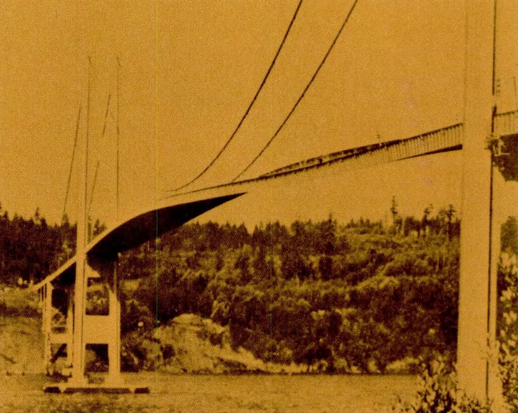
Engineers use the same reasoning on far larger systems. A bridge, a building or an aircraft wing has many natural ways of vibrating, called modes, which are eigenvectors of the matrices in its equations of motion, and the eigenvalues give how fast each mode oscillates and whether it dies away. The first Tacoma Narrows Bridge in Washington State, opened on 1 July 1940, collapsed on 7 November 1940 in winds of about 64 km/h, when a twisting motion of its deck kept growing instead of dying away. Engineers still debate the exact mechanism. The usual explanation is aeroelastic flutter, a self-exciting effect rather than simple resonance, in which the wind made the damping of the twisting mode effectively negative. Long-span bridge designs have since been tested to make sure that every mode stays damped at the wind speeds the bridge can expect.

Ranking web pages

The PageRank method behind early versions of Google's search engine, described by Sergey Brin and Larry Page in 1998, ranks web pages using a very large transition matrix. Each column describes a web user clicking from one page to the pages it links to, and the ranking of the pages is the eigenvector for eigenvalue 1, scaled so its entries add up to 1. It is the same calculation as the steady state of the two towns, applied to billions of pages; subtopic 3.15, Adjacency matrices, builds the matrix from a graph of links.

Exam focus

Eigenvalues and eigenvectors appear on Paper 1 and Paper 2 (and can be part of a Paper 3 investigation), usually as the opening parts of a longer question on a Markov chain (subtopic 4.19) or on coupled or second-order differential equations (subtopics 5.17 and 5.18). The eigenvalue and eigenvector parts are typically worth 5–8 marks together. The recurring shapes are:

• find the eigenvalues (characteristic equation, then roots): (M1)(A1)A1;

• find the eigenvectors: (M1) for an attempt at either, A1 for each, any non-zero multiple accepted unless a form such as integer entries is demanded;

• write down $P$ and $D$: one mark each, with a note that $P$ and $D$ must be consistent;

• hence find a long-term state or $M^n$

What to write down: the characteristic equation (the markscheme accepts any sign that $\det(M - \lambda I) = 0$ was used for the method mark), the two eigenvalues, the equation from $M - \lambda I$ used for each eigenvector, and the matrices $P$ and $D$

The "show that" in part (f) depends on writing every stage: the product $PD^nP^{-1}\boldsymbol{x}_0$, the inverse, $D^n$ and the final multiplication. Evaluating the formula at a couple of values of

When a question asks for $x$ as a function of $t$ or for one component of a vector, finish with that component in the form asked, for example "$a_n = \ldots$", not with the whole vector. When the command term is state, as in "state the long-term velocity", the answer follows from the eigenvalues alone and no further working is expected.

Practice questions

1. The matrix $A = \begin{pmatrix} 5 & -2 \\ 1 & 2 \end{pmatrix}$. Show that $\begin{pmatrix} 2 \\ 1 \end{pmatrix}$

Summary

• An eigenvector of a square matrix $M$ is a non-zero vector with $M\boldsymbol{v} = \lambda\boldsymbol{v}$; the eigenvalue $\lambda$ is the factor by which $M$ scales it. Any non-zero multiple of an eigenvector is also an eigenvector.

• Eigenvalues solve the characteristic equation $\det(M - \lambda I) = 0$

Self-check

• To do:

  I can check whether a vector is an eigenvector by multiplying it by the matrix.

• To do:

  I can explain why the zero vector is never an eigenvector.

• To do:

  I can derive $\det(M - \lambda I) = 0$ from $M\boldsymbol{v} = \lambda\boldsymbol{v}$.