4.5 Concepts of probability

Probability is the branch of mathematics that measures uncertainty. It assigns to every possible event a number between $0$ and $1$ that describes how likely the event is, so that chance can be reasoned about with the same precision as length or mass. Probability models are used to set insurance premiums, to judge whether a new medicine works better than an old one, to forecast the weather and to control the quality of manufactured goods.

The ideas introduced here form the vocabulary for all later work on probability: combining events with diagrams, conditional probability, and random variables such as the binomial and normal distributions.

Trials, outcomes and sample spaces

The language of probability

Probability describes situations whose result cannot be predicted with certainty: tossing a coin, rolling a die, choosing a person at random from a crowd, testing whether a light bulb is faulty. Each of these is a trial, and each possible result of the trial is an outcome. Exactly one outcome occurs every time the trial is carried out.

The sample space is written as a list of outcomes inside curly brackets. For one roll of an ordinary six-sided die,

The event "the score is even" is the set $A = \{2, 4, 6\}$, so $n(A) = 3$. An event occurs when the outcome of the trial is one of the outcomes in it: a roll of $4$ means that $A$ has occurred, and a roll of $5$ means that it has not.

Listing a sample space systematically

When a trial has several stages, such as tossing a coin more than once, the outcomes must be listed in an order that guarantees none is missed or repeated. A common method is to fix the first stage and run through every possibility for the later stages, then move to the next value of the first stage.

For two tosses of a coin, writing H for heads and T for tails, the outcomes are

The outcomes HT and TH are different: in HT the first toss shows heads, and in TH the first toss shows tails. Treating them as one outcome ("one head and one tail") would make the sample space wrong and every probability calculated from it incorrect.

Larger sample spaces, such as the $36$ outcomes when two dice are rolled, are easier to organise in a grid or a tree than in a list. These diagrams are developed in 4.6.

The probability of an event

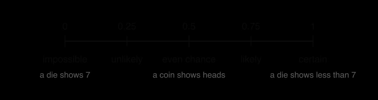
The probability scale

The probability of an event $A$ is written $P(A)$. It is always a number from $0$ to $1$ inclusive:

An event that cannot happen, such as rolling a $7$ on an ordinary die, has probability $0$. An event that is certain to happen, such as rolling a score less than $7$, has probability $1$. Probabilities may be written as fractions, decimals or percentages, so $\frac{1}{4}$, $0.25$ and $25\%$ all describe the same chance.

Equally likely outcomes

Many simple trials have outcomes that all have the same chance of occurring. A fair die is equally likely to land on any of its six faces, and a card shuffled into a well-mixed pack is equally likely to be any of the cards. In this situation the probability of an event is the fraction of the outcomes that belong to it.

This formula gives a theoretical probability: it comes from reasoning about the trial, not from carrying it out. The phrase "at random" in a question means that every item has the same chance of being chosen, so it signals that the outcomes are equally likely. Words such as "fair" (a fair coin, a fair die) and "unbiased" mean the same.

Simplifying a fraction does not change the probability, and either form is correct. A simplified fraction makes it easier to compare probabilities and to spot errors.

Problems with an unknown number of outcomes

Some questions give a probability and ask for the number of items that produces it. Setting $\frac{n(A)}{n(U)}$ equal to the given probability produces an equation that can be solved for the unknown.

Counting outcomes in a range of numbers

When a whole number is chosen at random from a range, the sample space is the list of whole numbers in that range. Counting the outcomes in the event carefully is the main step, and writing them out is the safest way to do it.

Complementary events

For any event $A$, the event "$A$ does not occur" is written $A'$ and read "$A$ prime" or "not $A$". It contains every outcome in the sample space that is not in $A$.

The Venn diagram shows why. The sample space $U$ is the rectangle, the event $A$ is the circle, and $A'$ is everything else. Every outcome lies in exactly one of the two regions, so $n(A) + n(A') = n(U)$. Dividing by $n(U)$ gives $P(A) + P(A') = 1$ when the outcomes are equally likely, and the result holds for all probabilities.

Rearranging gives the form used most often:

This is useful whenever the complement is easier to count than the event itself, as in the next example.

The complement of a complement

The complement of $A'$ is $A$ itself, written $(A')' = A$. The complement of the whole sample space is the empty event, which has probability $0$. These facts follow from the definition and are used when simplifying expressions with Venn diagrams in 4.6.

Experimental probability and relative frequency

Relative frequency

Theoretical probability relies on knowing that the outcomes are equally likely. For many real trials this is not true or cannot be checked: a drawing pin may land point up or on its side, a basketball player may score or miss a free throw, a manufactured part may or may not be faulty. In these cases the probability is estimated by carrying out the trial many times and recording how often the event occurs.

A relative frequency is always between $0$ and $1$, like a probability. It depends on the particular trials carried out, so two experiments usually give slightly different relative frequencies for the same event, while the true probability stays fixed.

A drawing pin dropped onto a table lands either point up or on its side, and there is no reason to expect these two outcomes to be equally likely. A student drops a pin repeatedly and records the running total of the times it lands point up.

Theoretical and experimental probability

The two kinds of probability answer the same question in different ways.

Experimental results can also be used to test a theoretical model. If a die is rolled $600$ times and a six appears $160$ times, the relative frequency $\frac{160}{600} \approx 0.267$ is far from $\frac{1}{6} \approx 0.167$. This is evidence that the die is biased, and the assumption of equally likely outcomes should be questioned. A small difference, on the other hand, is expected even for a fair die.

The law of large numbers

When a trial is repeated only a few times, the relative frequency can be far from the true probability. As the number of trials increases, the relative frequency tends to settle down and get closer to the probability. This result is called the law of large numbers.

The graph shows two simulated runs of $1000$ rolls of a fair die, with the relative frequency of a six recalculated after every roll. For the first fifty or so rolls both runs swing widely, between $0$ and more than $0.3$. After several hundred rolls both stay close to $\frac{1}{6}$.

A real experiment shows the same behaviour. The mathematician John Kerrich tossed a coin $10\,000$ times while interned during the Second World War. After $100$ tosses he had $44$ heads, a relative frequency of $0.44$; after all $10\,000$ tosses he had $5067$ heads, a relative frequency of $0.5067$.

Source: J. E. Kerrich, An Experimental Introduction to the Theory of Probability (1946).

The law describes the long run only. The number of heads did not become exactly half of the tosses: after $10\,000$ tosses Kerrich had $67$ more heads than half. The proportion of heads gets closer to $0.5$, even though the difference between the count and half the tosses need not shrink.

Simulations

Some probabilities are hard to calculate and slow or expensive to measure directly. A simulation imitates the real trial with random numbers, generated by a calculator, a computer, a table of random digits, dice or coins. Repeating the simulated trial many times gives a relative frequency that estimates the probability.

To design a simulation:

1. Assign random numbers to the outcomes so that their probabilities match the real situation.

2. Decide what counts as one trial and what counts as the event occurring.

3. Carry out many trials, and record whether the event occurs in each.

4. Calculate the relative frequency of the event.

Simulations are an example of mathematical modelling. The result can only be as good as the model: if births were not equally likely to be boys and girls, the simulation would need a different assignment of digits, such as $000$ to $511$ for boys out of $000$ to $999$.

Expected number of occurrences

If a fair die is rolled $600$ times, about one-sixth of the rolls are expected to show a six, which is $100$ sixes. In general, if an event has probability $p$ on each trial, the long-run proportion of trials in which it occurs is $p$, so in $n$ trials it is expected to occur about $np$ times.

The expected number is a long-run average, not a prediction of the exact count. Rolling a die $600$ times will rarely give exactly $100$ sixes, but if the $600$ rolls were repeated many times, the average number of sixes would be close to $100$. For the same reason the expected number does not have to be a whole number.

Expected numbers from relative frequencies

When the probability is unknown, a relative frequency can be used in its place. This is how factories estimate the number of faulty items in a large batch from a small sample, and how insurers predict the number of claims they will receive.

Finding the number of trials or the probability

The formula $np$ links three quantities, so knowing any two of them gives the third. Questions may give the expected number and ask for $n$ or for $p$.

Exam-style questions on probability concepts

Questions on these ideas are often short and are usually set where a graphic display calculator (GDC) is not allowed, so fractions should be handled confidently by hand. They also appear as the first parts of longer questions on combined events or random variables.

A typical short question gives a table of probabilities with an unknown, such as this one for a spinner with four coloured sections.

Longer questions combine counting with a parameter and the expected number formula. The following example is the kind of question that opens a longer probability problem.

When a question uses "show that", the final line must match the given value, and every step leading to it must be written. Starting from the given answer and checking that it works ($\frac{8}{20} = \frac{2}{5}$) is a verification, not a proof, and does not earn full credit.

Self-check

• To do:

  I can describe a trial, its outcomes, its sample space and an event, and list a sample space systematically.

• To do:

  I can use $P(A) = \frac{n(A)}{n(U)}$ when the outcomes are equally likely, and recognise when they are not.

• To do:

  I can find an unknown number of items from a given probability.

• To do:

  I can use $P(A') = 1 - P(A)$, including for "at least one" problems.

• To do:

  I can calculate a relative frequency and explain why more trials give a better estimate of a probability.

• To do:

  I can explain the difference between theoretical and experimental probability, and describe the law of large numbers.

• To do:

  I can design and carry out a simple simulation to estimate a probability.

• To do:

  I can calculate the expected number of occurrences $np$ and find $n$ or $p$ when the expected number is given.

choose a starting loaf at random from loaves 1 to 25, then select every 25th loaf after it R1

Note: The R1 requires both the random start and the regular interval.

Multiply both sides by $3(5 + x)$.

Check: $\frac{5}{15} = \frac{1}{3}$.

(b) Let $g$ be the number of green counters. The bag now holds $15 + g$ counters, still with $5$ red.

So $5$ green counters were added.

(b) Count the digits from $0$ to $4$ in each family. The families with at least two such digits are

That is $6$ families out of $20$.

(c) The estimate $0.3$ is well below the theoretical value $0.5$. With only $20$ simulated families, a large difference like this can easily happen by chance. By the law of large numbers, simulating many more families (several hundred, for example) would give a relative frequency closer to the true probability.

(b) Solve $160p = 36$.

The probability of not landing on red is $1 - 0.225 = 0.775$, so in $500$ spins the expected number is

Every step is shown, because "show that" means the given answer must be reached by working.

(b) $P(\text{odd}) = \frac{2}{5}$, so the expected number is (M1)

(c) The box now holds $24$ discs, of which $20 - 8 = 12$ are even. (M1 for the new totals)