Draw and describe scatter diagrams, find and interpret Pearson's r, fit a line of best fit through the mean point, and use the regression line of y on x to make sensible predictions.
Each is in the Maths AA glossary, with every other term in the subject.
Data in which two variables are measured or recorded for each individual or item, giving pairs of values that can be plotted and compared.
A relationship in which a change in one variable directly produces a change in another. Correlation alone never shows causation: both variables may depend on a third, or the link may be coincidence.
The square of Pearson's correlation coefficient, with
31 exam-style questions on this subtopic, written in the style of the IB papers. The first has its markscheme open. Counted on
A school has 570 students in three year groups, as shown in the following table.
Year group | 10 | 11 | 12 |
|---|---|---|---|
Number of students | 210 | 195 | 165 |
The school wants to investigate the relationship between screen time and sleep. It chooses a stratified sample of 40 students, proportional to the size of each year group.
Find the number of students from each year group in the sample, so that the total is exactly 40.
3 marks
attempt to find
One of 37 short multiple-choice questions on 4.4. Pick an answer to see why it's right or wrong.
The regression line of on is . How should be estimated when
With a free account, Augment remembers where you stopped and what you have practiced.
A relationship between two variables in which one tends to increase (positive correlation) or decrease (negative correlation) as the other increases. Linear correlation is when the points lie close to a straight line.
Using a regression line to predict a value outside the range of the data used to find it. Predicting inside that range is interpolation, which is much more reliable.
In bivariate data, the variable that is controlled or used to make predictions, plotted on the horizontal axis. The dependent variable is the one predicted, plotted on the vertical axis.
The point whose coordinates are the means of the two variables in a set of bivariate data. Every regression line and every good line of best fit passes through it.
A number , with , measuring the strength and direction of the linear correlation between two variables. Values near show strong linear correlation; values near show little or none.
The least squares line that makes the sum of the squares of the vertical distances from the data points to the line as small as possible. It passes through the mean point .
The difference between an observed value and the value predicted by a regression line, for the line of on ; on a scatter diagram it is the vertical distance from a point to the line.
A graph of bivariate data in which each pair of values is plotted as a single point, used to see whether and how the two variables are related.
Find the equation of the regression line of on with a GDC and interpret and in in context.
Use the regression line to make predictions, and decide whether a prediction is reliable (interpolation or extrapolation).
Decide whether a linear regression model is appropriate for a set of data.
Many questions in science, economics and everyday life are about how two quantities are related: whether heavier cars use more fuel, whether a house uses less gas in warmer weather, whether richer countries have longer life expectancies. Answering them needs data in which both quantities are recorded for each individual, and tools for measuring how closely the two are linked.
Linear correlation measures how close the points of such data lie to a straight line, and linear regression finds the equation of the best straight line through them. Together they turn a cloud of points into a linear model that can be used to make predictions, with a clear sense of how far those predictions can be trusted.
Most of the statistics in 4.2 and 4.3 is about a single variable, such as the heights of a group of students. When two variables are recorded for each member of a group, the data are bivariate. Each individual then gives an ordered pair .
Examples include the weight and fuel consumption of each of a set of car models, the outside temperature and gas used by a house in each of several weeks, and the height of each father and his adult son. The pairing matters: the values in each pair belong to the same individual, so the two lists cannot be reordered separately.
In a bivariate study one variable is often used to explain or predict the other. The independent variable is the one that is controlled, or that is known first and used to make predictions. The dependent variable is the one that responds to it, or that is to be predicted.
When neither variable clearly depends on the other (for example, the lengths of a person's left and right feet), either can be placed on the horizontal axis. The choice then depends on which variable is to be predicted from the other.
A scatter diagram shows bivariate data as a set of points, one for each pair. The pattern of the points shows at a glance whether the variables are related and how.
To draw a scatter diagram by hand:
Put the independent variable on the horizontal axis and the dependent variable on the vertical axis.
Choose a scale for each axis that covers the range of the data and uses most of the grid. An axis does not need to start at .
Label both axes with the variable and its units.
Plot each pair as a small cross or dot. Do not join the points and do not draw a line yet.
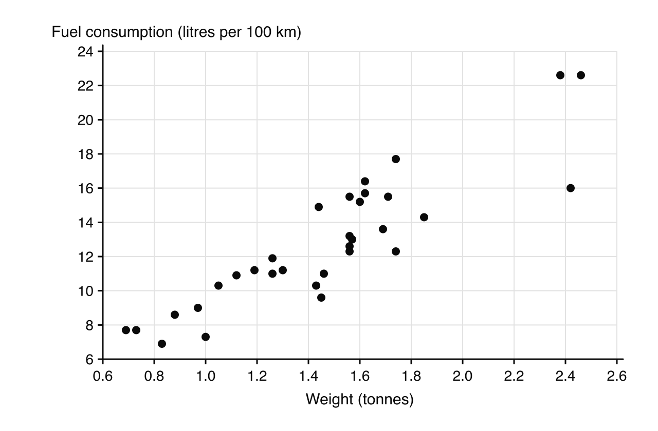
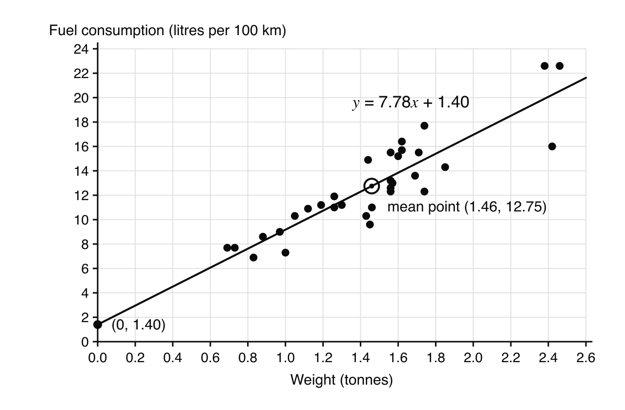
In the scatter diagram of 32 car models tested in the 1970s, each point is one car, with its weight across and the fuel it uses to travel 100 km up.
When the points on a scatter diagram follow a trend, the variables show correlation. A full description of the correlation covers three features.
Direction: positive (the points rise from left to right), negative (they fall) or no correlation (no trend).
Form: linear (the points cluster around a straight line) or non-linear (they follow a curve).
Strength: strong if the points lie close to the line or curve, weak if they are widely scattered about it.
Six scatter diagrams show the most common patterns. In the last one the variables are closely related, but the relationship is a curve rather than a line, so there is no linear correlation.

A point that lies well away from the overall pattern is an outlier. On a scatter diagram an outlier need not be extreme in either variable on its own: a car of average weight with very low fuel consumption would stand out only because of the combination of its values. Outliers should be checked, since they may be recording errors, but they should not be deleted just because they do not fit. Points can also form separate clusters, which often means the data contain two different groups (for example, cars with petrol engines and cars with diesel engines).
Words such as "strong" and "weak" are a matter of judgement. Pearson's product-moment correlation coefficient, written , puts a number on the strength and direction of a linear correlation.
Its key properties are:
means every point lies exactly on a straight line with a positive gradient; means every point lies on a line with a negative gradient. These are perfect correlations.
The sign of gives the direction of the correlation, and the size gives its strength.
close to means there is little or no linear correlation. It does not rule out a curved relationship.
has no units. Changing units (centimetres to inches, or kilograms to pounds) does not change it, and neither does swapping the roles of and .
is sensitive to outliers. A single point far from the rest can make it much larger or much smaller.
The value of is found with a graphic display calculator (GDC). Its formula involves sums of products of deviations from the mean, which is where the name "product-moment" comes from, but it is never calculated by hand in this course.
Different books use slightly different boundaries, but the descriptions in the table are widely accepted and are a sound rule of thumb.
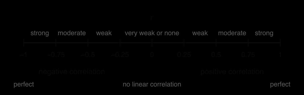
Value of | Description |
|---|---|
or | perfect positive or perfect negative linear correlation |
strong | |
moderate | |
weak | |
very weak or no linear correlation |
For the 32 cars, a GDC gives (3 s.f.), confirming the strong positive linear correlation seen on the scatter diagram.
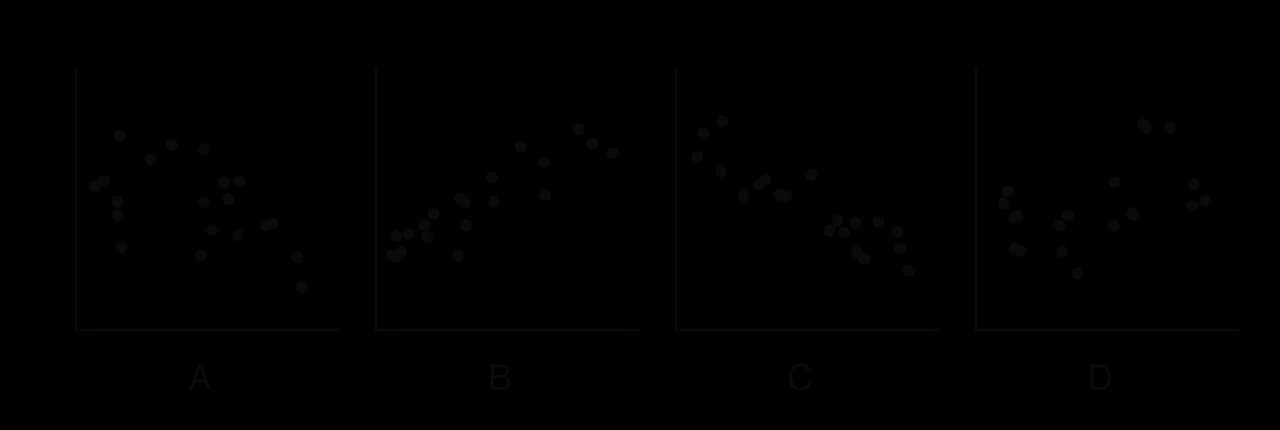
The scatter diagrams A to D show four correlations of different directions and strengths.
On any GDC the steps are the same in outline:
Enter the -values in one list and the corresponding -values in a second list, keeping each pair in the same row.
In the statistics menu, choose two-variable statistics or linear regression of the form .
Read off (and, for regression, and ). On some models is shown only after a "diagnostics" or "statistics display" setting has been switched on.
Squaring gives the coefficient of determination . It is not needed for every question, but it gives a useful interpretation of the strength of a correlation.
For the cars, : about of the variation in fuel consumption between the 32 cars is accounted for by the differences in their weight. The remaining comes from other factors, such as engine size and design.
A strong correlation between two variables does not show causation, that is, that changing one variable produces a change in the other.
There are three common reasons why two variables can be correlated without one causing the other.
A third variable. Both variables may depend on something else, sometimes called a lurking or confounding variable. Across a summer, ice-cream sales and the number of people needing rescue at beaches rise and fall together because both increase in hot weather.
Reverse direction. The cause may run the other way from the one suggested. Cities with more police officers tend to have more crime, but mostly because cities with more crime employ more police.
Coincidence. Any two quantities that both grow over the same period, such as a country's mobile-phone use and the average height of its children, will be correlated even if they have nothing to do with each other.
Causation can be established only by other means, usually a controlled experiment in which one variable is changed deliberately while everything else is kept the same.
When a scatter diagram shows linear correlation, a straight line drawn through the middle of the points summarises the trend. Such a line of best fit can be drawn by eye, or found exactly as the regression line.
The means of the two variables give a single point at the centre of the data.
The mean point is the balance point of the data, and every good line of best fit passes through it. Plot it first, marked differently from the data points (for example with a circle), and draw the line through it.
Calculate the mean point and plot it.
Place a ruler through the mean point and turn it until it follows the trend, with roughly equal numbers of points on each side along the whole line (not all of one side's points at one end).
Draw the line across the range of the data only.
To find its equation, read the coordinates of a second point on the line, far from the mean point, and use the methods of 2.1: the gradient from the two points, then .
A line drawn by eye depends on the person drawing it, so two people will usually get slightly different equations. It is useful for a quick estimate, or when no GDC is available.
A house owner recorded the average outside temperature, °C, and the gas used to heat the house, thousand cubic feet, for ten weeks of one winter.
(°C) | ||||||||||
|---|---|---|---|---|---|---|---|---|---|---|
(thousand ft³) |
Data: D. Whiteside, UK Building Research Station, house in south-east England, 1960s (Hand et al., 1993).
To find a single best line that everyone agrees on, there needs to be a precise meaning of "best". For a line used to predict from , the errors that matter are the vertical distances between the points and the line, because these are the errors in .
For the ten weeks of gas data, the residuals are the vertical segments between the points and the regression line. Some are positive and some negative; for the best line they add up to .
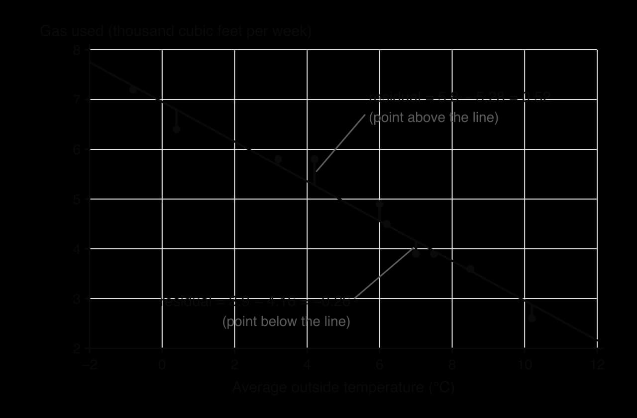
The least squares principle chooses the line that makes the sum of the squares of the residuals as small as possible. Squaring makes every term positive, so positive and negative errors cannot cancel, and it penalises large errors more heavily than small ones. The line found this way is the regression line of on .
The values of and come from formulas involving the means and sums of products of the data, but in this course they are always found with a GDC, in the same menu as . Different calculators may write the line as or , so check which letter is the gradient.
In the regression line , both coefficients have a meaning in context.
The gradient is the change in for each increase of one unit in , on average. Its units are "units of per unit of ".
The y-intercept is the predicted value of when . It has a sensible meaning only if is a realistic value that lies inside, or very close to, the range of the data.
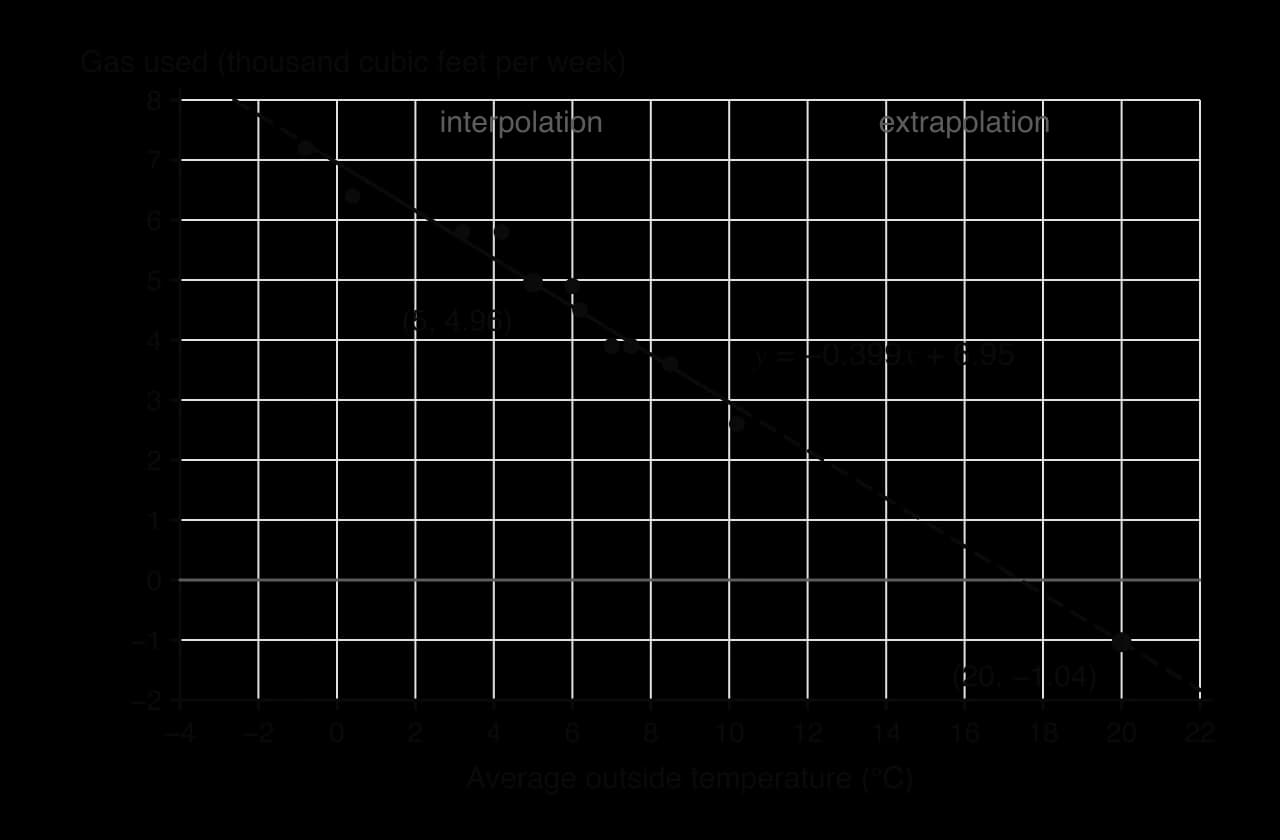
For the gas data, means that for each extra 1 °C of average outside temperature, the house uses about thousand cubic feet less gas per week. The intercept means that in a week with an average temperature of 0 °C the house would use about thousand cubic feet. Since 0 °C is inside the data range ( °C to °C), this is a meaningful prediction.
The regression line for the 32 cars, by contrast, has an intercept with no practical meaning.
Because the regression line always passes through , substituting into its equation always gives . This allows questions without a GDC in which a mean or a missing data value is found from the equation of the line.
The main use of a regression line is prediction: substitute a value of to estimate . How far a prediction can be trusted depends on where the value of lies.
Interpolation is usually reliable when the correlation is strong, because the data show that the linear pattern holds there. Extrapolation assumes the same straight line continues beyond the data, and there is no evidence for that. Many real relationships level off, curve or stop making sense outside the range observed, so extrapolated predictions can be badly wrong even when is very close to .
The regression line of on is designed to predict . It minimises the errors in , not in , so rearranging it to predict from a given does not in general give the best estimate. To predict from , a different line is used, the regression line of on , which is covered in 4.10. The two lines are the same only when .
A GDC will produce a value of and a regression line for any set of pairs, whether or not a straight line makes sense. Before using a regression line, check the scatter diagram and the value of .
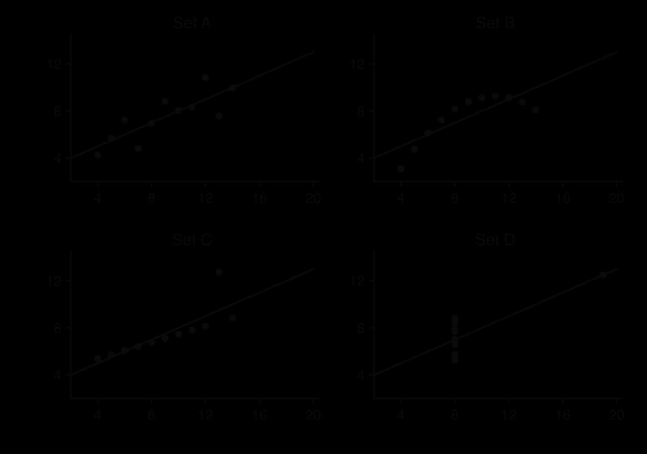
Anscombe's quartet is a set of four small data sets constructed in 1973 to show why. All four have the same means, the same correlation coefficient () and the same regression line, (to 2 significant figures), yet they look completely different.
Real data can show the same problem as set B. Across the world, life expectancy rises with national income, but not in a straight line: among the poorest countries a small increase in income goes with a large increase in life expectancy, while among rich countries extra income makes little difference.
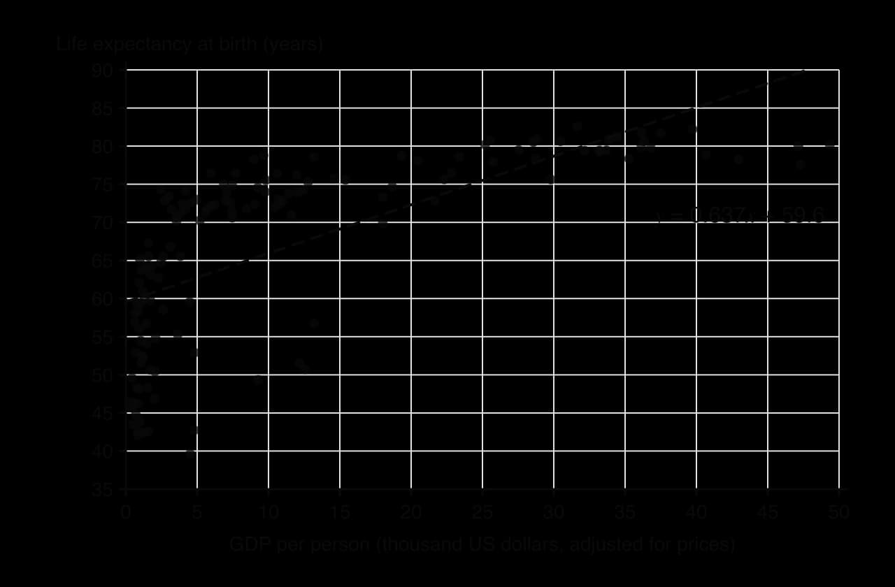
For these 142 countries , a moderate positive correlation, and the regression line of life expectancy on GDP per person (in thousands of dollars) is . The value of alone would suggest a reasonable linear model, but the scatter diagram shows that the line overestimates life expectancy for the poorest and the richest countries and underestimates it for many countries in between. A prediction from this line would be systematically wrong, however carefully it was calculated.
A regression line of on is appropriate for prediction when:
the scatter diagram shows a linear pattern, with no clear curve;
the correlation is strong (as a rough rule, ; with a moderate correlation predictions are much less precise);
there are no outliers or isolated points controlling the line;
the prediction is of from a value of (otherwise use on , in 4.10);
the value of is inside the range of the data (interpolation).
Questions on this subtopic usually appear on the calculator paper, with data given in a table. Parts typically ask for , a description of the correlation, the regression line, a prediction, and a comment on the reliability of a prediction or on causation. Questions without a GDC give the equation of the line, or , and test interpretation and the mean point.
The table gives GDP per person, thousand US dollars, and life expectancy at birth, years, for ten European countries in 2007.
Country | ||
|---|---|---|
Albania | ||
Turkey | ||
Romania | ||
Poland | ||
Hungary | ||
Portugal | ||
Czech Republic | ||
Greece | ||
Germany | ||
Ireland |
Data: Gapminder, 2007.
I can draw a scatter diagram with the independent variable on the horizontal axis and describe the correlation by direction, form and strength, in context.
I can find with a GDC and describe its value in words, and I know that measures linear correlation only.
I can explain, with an example of a third variable, why correlation does not show causation.
I can calculate the mean point and draw a line of best fit by eye through it.
I can find the regression line of on with a GDC and interpret its gradient and -intercept in context.
I can use the fact that the regression line passes through to find a missing mean or data value.
I can make a prediction from the regression line and say whether it is interpolation or extrapolation and how reliable it is.
I can decide from the scatter diagram and whether a linear regression model is appropriate.
(A1)
rounding to the nearest integer gives a total of 41, so one group must be rounded down
Year 10: 15, Year 11: 14, Year 12: 11 A1
Note: Accept any choice of three integers totalling 40 with each within 1 of the exact values, provided the student explains the adjustment, e.g. 15, 13, 12. Award A0 for 15, 14, 12.
Suggest one reason why a stratified sample is suitable for this investigation.
1 mark
students in different year groups may have different amounts of screen time and sleep, so each year group should be represented in proportion R1
Eight of the sampled students recorded their mean daily screen time, hours, and their mean nightly sleep, hours, over one week. The results are shown in the following table.
1.5 | 2.0 | 3.2 | 4.0 | 4.8 | 5.5 | 6.1 | 7.0 | |
|---|---|---|---|---|---|---|---|---|
8.9 | 8.6 | 8.1 | 7.9 | 7.2 | 7.0 | 6.6 | 6.1 |
Find Pearson's product-moment correlation coefficient, , for these data.
2 marks
A2
The regression line of on is . Find the value of and the value of .
2 marks
A1
Use the regression line to estimate the mean nightly sleep of a student whose mean daily screen time is 3.5 hours.
2 marks
(M1)
(hours) A1
Note: Accept or from using 3 s.f. values of and .
A teacher claims that these results prove that more screen time causes students to sleep less. Comment on this claim.
1 mark
a strong (negative) correlation does not show causation (other factors such as homework or age could affect both; and the sample is only 8 students) R1
Explain why the regression line should not be used to estimate the sleep of a student whose mean daily screen time is 11 hours.
1 mark
11 hours is outside the range of the data (), so this would be extrapolation R1
Three of the 40 students selected did not return their questionnaires. Explain why this missing data could make the results less reliable.
1 mark
students who did not respond may differ from those who did (e.g. they may have much more screen time), so the remaining data may not be representative R1
A librarian surveys a group of students. For each student, the number of hours spent reading each week, , and their score in a reading test, , are recorded.
For these data, the regression line of on is and the regression line of on is .
One of the students reads for 8 hours each week. Use an appropriate regression line to estimate this student's score in the test.
2 marks
Another student scored 70 in the test. Use an appropriate regression line to estimate the number of hours this student reads each week.
2 marks
State whether Pearson's product-moment correlation coefficient for these data is positive or negative. Give a reason for your answer.
1 mark
The members of a running club record their resting heart rate, beats per minute, and the time, minutes, that they take to run 1 km.
For these data, the regression line of on is and the regression line of on is .
Find the mean resting heart rate and the mean time to run 1 km for the members of the club.
4 marks
One member of the club has a resting heart rate of 52 beats per minute. Use an appropriate regression line to estimate the time this member takes to run 1 km.
2 marks
Use the regression line of on
Substitute into the line
Rearrange the line to get
Use , since is the same either way
It does not. A strong correlation shows only that the two variables tend to change together. Other factors, such as how much the students revised (students who revise more may have less time for their phones), could explain both.
3. The line by eye, , has almost the same gradient and intercept. Both pass through the mean point: for the regression line,
The regression line is the one that would be produced by anyone with the same data, which is why it is preferred.
3. tonnes lies inside the data range, so substitute (using the unrounded values , from the GDC):
A car weighing 1.5 tonnes is expected to use about litres per 100 km.
The regression line passes through , so
The five -values must therefore add up to :
4. For each additional thousand dollars of GDP per person, life expectancy increases by about years (roughly 2.4 months) on average.
5. is inside the data range ( to ), so substitute the unrounded values:
6.
This is unreliable: is outside the range of the data ( to ), so it is extrapolation. The correlation is also only moderate. (Norway's actual life expectancy in 2007 was 80.2 years, lower than the prediction: among the richest countries life expectancy levels off.)
7. The line is the regression line of on , which is designed to predict from . Estimating from needs the regression line of on .
The café sells a mean of hot drinks per day.
2. For each 1 °C increase in maximum temperature, the café sells about fewer hot drinks on average.
3. °C lies inside the range 8 °C to 28 °C:
About hot drinks.
4. °C is outside the range of temperatures recorded, so the prediction is an extrapolation and there is no evidence that the linear pattern continues. In fact the line gives , a negative number of drinks, which is impossible.
5. . About of the variation in the number of hot drinks sold is accounted for by the linear relationship with temperature.