4.3 Measures of central tendency and dispersion · IB Maths AA | Augment Education
4.3 Measures of central tendency and dispersion
Calculate the mean, median, mode, quartiles, range, IQR, variance and standard deviation of raw, discrete and grouped data, predict the effect of adding or multiplying by a constant, and choose the most suitable measures.
IB Mathematics: Analysis and Approaches
Part of 4 Statistics and probability
SL and HL
Key terms introduced here
Each is in the Maths AA glossary, with every other term in the subject.
Notes on 4.3 Measures of central tendency and dispersion
29 min readLast reviewed
A single number can often summarise a whole data set well enough to compare it with another or to make a decision. Two kinds of number are needed: one that describes where the data are centred (a typical value) and one that describes how spread out they are. Two classes with the same mean test score can be very different if one class has scores clustered tightly around the mean and the other has scores ranging from very low to very high.
Questions on 4.3
48 exam-style questions on this subtopic, written in the style of the IB papers. The first has its markscheme open. Counted on
Question 1 · AA-003856 marks
A biology student grows 12 tomato seedlings for three weeks and then records the height of each seedling, in cm. The recorded heights are shown below.
0.64.85.25.55.96.16.46.67.07.37.911.8
A value is considered an outlier if it is more than 1.5×IQR
Try a quick-fire question
One of 40 short multiple-choice questions on 4.3. Pick an answer to see why it's right or wrong.
The values 0, 1, 2 and 3 have frequencies 4, 3, 2 and 1. What is the mean?
From the formula booklet
The entries of the mathematics: analysis and approaches formula booklet that 4.3 uses. Each opens in the explained booklet.
The mean of the squared deviations from the mean, σ2=n∑f(x−μ)2. Its units are the square of the data's units.
, is in 4.7. In this course the standard deviation of data is found with the GDC, and the population standard deviation
σ
is used throughout.
Measures of central tendency
A measure of central tendency is a single value that represents the centre of a data set. The three in common use are the mean, the median and the mode, and each describes "typical" in a different way.
The mean
The mean is the familiar "average": add all the values and divide by how many there are. For n values x1,x2,…,xn, the mean is written xˉ (read "x bar"):
xˉ=n∑i=1nxi
When the data are the whole population, the mean is often written μ instead. The two symbols are calculated in the same way.
The mean uses every value in the data. It is the balance point of the data: if the values were equal weights on a ruler, the ruler would balance at the mean. The deviations from the mean, x−xˉ, always add up to zero, which is why the mean lies between the extremes and is pulled towards any value far from the rest.
The median
The median is the middle value once the data are in order. For n values it is the 2n+1th value: when n is odd this is a single value, and when n is even it is halfway between the two middle values.
Half of the data lie on each side of the median. Only the order of the values matters, not their sizes, so changing the largest value from 25 to 2500 does not change the median at all.
The mode
The mode is the most frequent value. It is the only average that can be used for qualitative data (the most common blood group, the most popular colour), and it is useful when the most common value matters, such as the shoe size a shop should stock most of.
A data set with two modes is bimodal. If every value occurs once, there is no mode.
Data in a frequency table
When each value x occurs with frequency f, the sum of all the data is ∑fx and the number of data is n=∑f. The mean is
xˉ=n∑i=1kfixi,n=i=1∑kfi
where k is the number of different values. The median is still the 2n+1th value, found by counting through the frequencies, and the mode is the value with the highest frequency.
In a study of 189 births, each mother was asked how many times she visited a physician during the first three months of pregnancy. The results are in the table.
Number of visits, x
0
1
2
3
4
6
Frequency, f
100
47
30
7
4
1
Data: low birth weight study, Baystate Medical Center, Springfield, Massachusetts, 1986 (Hosmer and Lemeshow).
Grouped data: estimating the mean
When data are grouped into classes, the exact values are unknown. Each value is replaced by the mid-interval value of its class, which assumes the values in each class are spread evenly around its centre. The mean calculated this way is an estimate.
The class with the highest frequency is the modal class. For grouped data, the modal class takes the place of the mode, and the median is estimated from a cumulative frequency graph (see 4.2).
The waiting times between 272 eruptions of the Old Faithful geyser are grouped in the table, in classes of width 10 minutes.
Waiting time, t (minutes)
40≤t<50
50≤t<60
60≤t<70
70≤t<80
80≤t<90
90≤t<100
Frequency
21
56
26
77
80
12
Data: Old Faithful geyser, 272 eruptions (Härdle, 1991).
Solving for unknown values
Many questions give the mean and ask for a missing value. The key fact is that the sum of the data equals the mean multiplied by the number of values:
∑x=nxˉ
The same idea works for an unknown frequency: write ∑fx and ∑f in terms of the unknown, form an equation with the given mean, and solve.
For example, the table shows the number of goals, x, scored by a team in each match of a season, with one frequency unknown.
Goals, x
1
2
3
4
Frequency, f
5
k
8
2
Combining two groups
The mean of two groups together is not the mean of the two means, unless the groups are the same size. The correct method combines the totals:
xˉcombined=n1+n2n1xˉ1+n2xˉ2
Quartiles of discrete data
The GDC method
Several slightly different rules for quartiles are used in different books and software. This course uses the rule built into a graphic display calculator (GDC):
Put the data in order and find the median.
Split the data into a lower half and an upper half. If n is odd, leave the median out of both halves. If n is even, the halves are the first 2n and the last 2n values.
Q1 is the median of the lower half, and Q3 is the median of the upper half.
For large data sets, the GDC's one-variable statistics give Q1, the median and Q3 directly, and these are the values to use.
For a frequency table, count through the frequencies to find the positions. For the 189 physician-visit values, the median is the 95th value (0). The lower half is the first 94 values, whose median is between the 47th and 48th values, both 0, so Q1=0. The upper half is the 96th to 189th values; its middle values are the 142nd and 143rd values of the whole list, which lie among the values equal to 1 (positions 101 to 147), so Q3=1.
Measures of dispersion
Why spread matters
A measure of dispersion describes how spread out the data are. Two data sets can have the same mean and still be very different. The data sets A: 4,5,6,6,7,8 and B: 1,3,6,6,9,11 both have mean 6 and median 6, but the values of B lie much further from the centre.
Range and interquartile range
The range is the simplest measure of spread.
The range is easy to find but depends only on the two most extreme values, so a single outlier can make it very large. The interquartile range, IQR=Q3−Q1, measures the spread of the middle half of the data and ignores the extremes (it is defined in 4.2). It is the natural partner of the median.
Variance and standard deviation
The range and IQR each use only two values. A measure that uses every value starts from the deviationsx−μ, the distances of the values from the mean. Their plain average is always zero, because positive and negative deviations cancel. Squaring them first makes every term positive, and averaging the squares gives the variance, σ2.
The variance is measured in squared units (cm² for heights in cm), which is hard to interpret. Its square root, the standard deviation σ, is in the same units as the data, and is roughly the typical distance of a value from the mean.
Both sets have mean 6. The deviations in set B are larger, so its standard deviation is larger: about 3.37 against 1.29.
A small standard deviation means the values cluster closely around the mean; a large one means they are widely scattered. A standard deviation of 0 means every value is the same. The standard deviation is never negative.
A second form of the variance
Expanding the squared deviation gives a form that is often quicker to use by hand. Since ∑f=n and ∑fx=nμ,
In words, the variance is the mean of the squares minus the square of the mean.
Standard deviation with a GDC
In practice the standard deviation is found with a GDC. Enter the data in a list (with a second list for frequencies, if there is a table), then choose one-variable statistics. The GDC shows two standard deviations:
GDC symbol
Divides by
Use
σx
n
The standard deviation of the data: the one used in this course
sx
n−1
An estimate of a larger population's standard deviation from a sample; not used here
The two values are close for large data sets but can differ noticeably for small ones.
Interpreting the standard deviation
A standard deviation is interpreted by comparison: with the mean of the same data (is the spread large relative to the typical value?) or with the standard deviation of another data set measured in the same units. A smaller standard deviation means more consistent values. An interpretation should always be written in the context of the data, not only as a number.
The effect of constant changes
Adding a constant
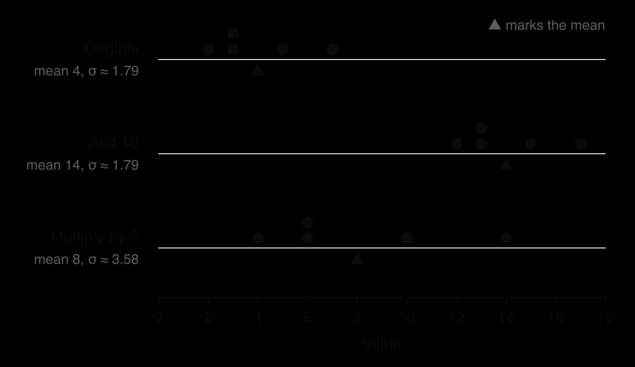
If the same number b is added to every value, the whole distribution slides along by b without changing shape. Every measure of centre moves by b, and every distance between values stays the same, so the measures of spread do not change.
Multiplying by a constant
If every value is multiplied by a positive number a, the whole distribution is stretched by a factor of a about 0. Every measure of centre is multiplied by a, and every distance between values, including every deviation from the mean, is multiplied by a. The standard deviation, range and IQR are therefore multiplied by a, and the variance, which is built from squared deviations, by a2.
Adding 10 moves the data along without changing the spread. Multiplying by 2 doubles the mean and doubles the spread.
The two effects combine. For a change y=ax+b with a>0:
Measure
Add b to every value
Multiply every value by a
Both: y=ax+b
Mean, median, mode, quartiles
+b
×a
yˉ=axˉ+b
Range, IQR, standard deviation
unchanged
×a
σy=aσx
Variance
unchanged
×a2
σy2=a2σx2
If a is negative, the order of the data is reversed but distances are still multiplied by ∣a∣, so σy=∣a∣σx and the variance is still multiplied by a2. The mean is axˉ+b in every case.
Choosing an appropriate measure
Effect of outliers and skewness
The mean uses the size of every value, so a few very large or very small values pull it towards them. The median depends only on the order of the values, so it is resistant to outliers. In the same way, the standard deviation and range are strongly affected by outliers, while the IQR is not.
In a symmetric distribution, the mean and median are equal or close. In a skewed distribution they separate, and the mean lies further along the tail:
Shape
Usual order
Symmetric
mean ≈ median ≈ mode
Positive skew (tail to the right)
mode < median < mean
Negative skew (tail to the left)
mean < median < mode
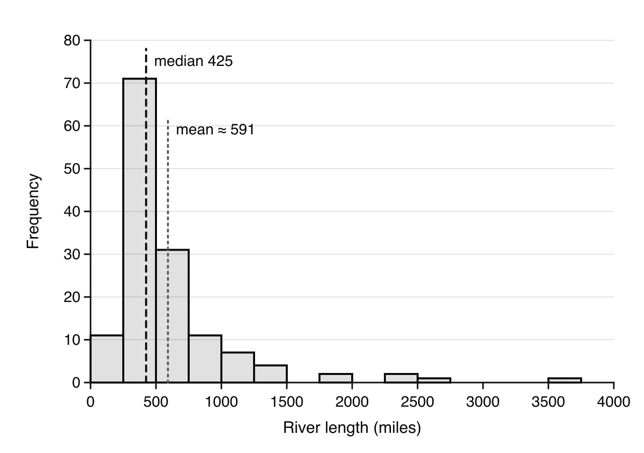
The long tail of very long rivers pulls the mean (591 miles) well to the right of the median (425 miles). Data: The World Almanac and Book of Facts (1975).
The river lengths are strongly positively skewed. Their mean, 591 miles, is larger than the lengths of two thirds of the rivers, so it does not describe a typical river well. The median, 425 miles, does. Similarly, the standard deviation, 492 miles, is inflated by the ten outliers, while the IQR, 378 miles, describes the spread of the typical rivers.
Guidelines
Situation
Measure of centre
Measure of spread
Roughly symmetric, no outliers
Mean
Standard deviation
Skewed, or with outliers
Median
Interquartile range
Qualitative data, or the most common value is wanted
Mode
(none)
Bimodal
Describe both peaks; no single average is typical
Describe the two groups
The mean and standard deviation are preferred when they are appropriate because they use every value and work well with further calculation (they are the parameters of the normal distribution in 4.9). The median and IQR are preferred when the data are skewed or contain outliers, which is why national statistics usually report median income rather than mean income.
The Old Faithful waiting times show the limits of any single average. Their mean (70.9 minutes) lies close to the trough between the two clusters of waits in the histogram in 4.2, where relatively few waits occur, and their median (76 minutes) sits at the lower edge of the larger cluster. Neither describes the short waits at all. A visitor is better told that the wait is usually either about 50 to 60 minutes or about 75 to 85 minutes.
Exam-style questions on measures of centre and spread
The birth weights of all 189 babies in the hospital study are grouped in the table.
Birth weight, w (grams)
Frequency
500≤w<1000
1
1000≤w<1500
4
1500≤w<2000
14
2000≤w<2500
40
2500≤w<3000
38
3000≤w<3500
45
3500≤w<4000
38
4000≤w<4500
7
4500≤w<5000
2
Data: 189 births, Baystate Medical Center, Springfield, Massachusetts, 1986 (Hosmer and Lemeshow).
Self-check
To do:
I can calculate the mean, median and mode of a list of data and of a frequency table.
To do:
I can estimate the mean of grouped data using mid-interval values, and write down the modal class.
To do:
I can find the quartiles of discrete data using the GDC method, for odd and even numbers of values.
To do:
I can calculate the range, IQR, variance and standard deviation, by hand for small data sets and with a GDC using σx.
To do:
I can use ∑x=nxˉ to find unknown values or frequencies, and combine the means of two groups.
To do:
I can state the effect of adding a constant, or multiplying by a constant, on each measure of centre and spread.
To do:
I can choose suitable measures of centre and spread for a data set, with reasons based on outliers and skewness.
below the lower quartile or more than
1.5×IQR
above the upper quartile.
(a)
Find the lower quartile and the upper quartile of the recorded heights.
[2]2 marks
Markscheme (a)
Q1=5.35A1
Q3=7.15A1
(b)
Show that 0.6 and 11.8 are both outliers.
[2]2 marks
Markscheme (b)
IQR=7.15−5.35=1.8(A1)
Q1−1.5×1.8=2.65
(c)
Every seedling was at least 3 cm tall when it was planted at the start of the three weeks. For each of the two outliers, state whether it should be kept in or removed from the data, giving a reason.
[2]2 marks
Markscheme (c)
0.6 should be removed: a seedling at least 3 cm tall cannot have a height of 0.6 cm three weeks later, so it must be an error in recording (e.g. a misplaced decimal point or a value in different units) R1
11.8 should be kept: it is possible for one seedling to grow much more than the others, so it is a valid (genuine) data value R1
Note: Award R1 for each correct decision with a valid reason. Do not award R1 for a decision without a reason.
Question 2 · AA-003896 marks
A courier records the masses, in kg, of nine parcels delivered on one morning.
2.403.851.9531.52.704.102.253.302.85
(a)(i)
For the recorded masses, find the mean.
[1]1 mark
(a)(ii)
For the recorded masses, find the standard deviation.
[1]1 mark
(b)
The courier then discovers that the mass of 31.5 kg was a recording error, and that the true mass of this parcel was 3.15 kg. Find the mean and the standard deviation of the nine true masses.
[2]2 marks
(c)
State, with a reason, whether correcting the error changes the median mass.
A town has 6400 households. An energy company selects a simple random sample of 250 of these households. Of the households in the sample, 48 have solar panels.
(a)
Estimate the number of households in the town that have solar panels.
[2]2 marks
(b)(i)
The daily electricity use, E kWh, of each household in the sample is recorded. The results are shown in the following table.
Daily use, E kWh
Number of households
0≤E<5
18
5≤E<10
52
10≤E<15
85
15≤E<20
61
20≤E<25
26
25≤E<30
8
Write down the modal class.
[1]1 mark
(b)(ii)
Find an estimate of the mean and an estimate of the standard deviation of the daily electricity use.
[3]3 marks
(c)
Estimate the number of households in the town that use at least 20 kWh per day.
[2]2 marks
(d)
The company contacts 12 households in the town, chosen at random. Assume that the proportion of all households in the town with solar panels is the same as the proportion in the sample. Find the probability that at least 3 of the 12 households have solar panels.
[3]3 marks
(e)
State one assumption required for the model used in part (d).
[1]1 mark
(f)
An employee suggests that it would have been quicker to survey the 250 households that live closest to the company's office. Give two reasons why this would be likely to give less reliable estimates than the random sample.
(b) n=10 (even). The median is halfway between the 5th and 6th values: 228+30=29.
Lower half (first five values): 21,23,23,26,28, so Q1=23.
Upper half (last five values): 30,31,35,36,40, so Q3=35.
IQR=35−23=12.
s,
σ=0.422
s (3 s.f.).
(b) The means are almost the same, so the sprinters are equally fast on average. Sprinter A's standard deviation is about a third of sprinter B's, so A's times are much more consistent: all five are within 0.2 s of the mean, while B's vary from 9.9 s to 10.9 s. A is the better choice for a steady time under 10.5 s, although B is more likely to run the single fastest time.
Mean: apply the whole conversion.
Cˉ=95(49.39−32)=95(17.39)=9.66°C (3 s.f.)
Standard deviation: only the multiplication affects the spread; subtracting 32 does not.
σC=95×8.243=4.58°C (3 s.f.)
Data: monthly mean air temperatures at Nottingham Castle, 1939 (Anderson, Time Series Analysis and Forecasting, 1976; the nottem data set in R).
, which is also
1.042×852=1.0816×7225=7814.56
(in USD², a unit that has no everyday meaning).
thousand dollars, which describes the spread of the typical salaries. The range (218) and the standard deviation (about 63.3) are both dominated by the single outlier.
.
[1]
xˉ≈2920g(2924.6…),σ≈743g(742.6…)
[2]
(c) Dividing every weight by 1000 divides the mean and the standard deviation by 1000:
xˉ≈2.92kg,σ≈0.743kg
[2]
(d) 1+4+14+40=59 babies weighed less than 2500 g. [1]
18959×100=31.2%(3 s.f.)
[1]
(e) IQR=3515.5−2412=1103.5 g. [1]
Lower boundary: 2412−1.5×1103.5=2412−1655.25=756.75 g. [1]
Since 709<756.75, the weight of 709 g is an outlier. [1]