4.2 Presenting data · IB Maths AA | Augment Education
4.2 Presenting data
Organise discrete and continuous data in frequency tables, draw and read histograms, cumulative frequency graphs and box-and-whisker diagrams, find quartiles, percentiles and outliers, and compare distributions.
IB Mathematics: Analysis and Approaches
Part of 4 Statistics and probability
SL and HL
Key terms introduced here
Each is in the Maths AA glossary, with every other term in the subject.
A diagram of a data set drawn on a scale: a box from Q1 to Q3 with a line at the median, and whiskers to the smallest and largest values that are not outliers.
A range of values used to group data, such as 50≤t<55
Notes on 4.2 Presenting data
25 min readLast reviewed
A list of 272 numbers says very little at a glance. Organised into a table and drawn as a diagram, the same numbers show at once where most values lie, how spread out they are, whether the distribution is symmetric, and whether any values are unusual. Choosing the right representation is a central skill in statistics, because each diagram makes some features visible and hides others.
Questions on 4.2
32 exam-style questions on this subtopic, written in the style of the IB papers. The first has its markscheme open. Counted on
Question 1 · AA-003856 marks
A biology student grows 12 tomato seedlings for three weeks and then records the height of each seedling, in cm. The recorded heights are shown below.
0.64.85.25.55.96.16.46.67.07.37.911.8
A value is considered an outlier if it is more than 1.5×IQR
Try a quick-fire question
One of 40 short multiple-choice questions on 4.2. Pick an answer to see why it's right or wrong.
What is the upper quartile of 3, 5, 6, 8, 9, 10, 12, 13, 15, 18, 20?
From the formula booklet
The entries of the mathematics: analysis and approaches formula booklet that 4.2 uses. Each opens in the explained booklet.
The running total of the frequencies up to a given value or upper class boundary. Plotted against the upper boundaries, it gives a cumulative frequency graph.
A diagram for grouped continuous data in which each class is drawn as a bar with no gaps between bars. With equal class widths, the height of each bar is the frequency.
One of the values that divide ordered data into four equal parts: the lower quartile Q1 has a quarter of the data below it, the upper quartile Q3 three quarters.
The lack of symmetry in a distribution. A positively skewed distribution has a long tail to the right (high values); a negatively skewed one has a long tail to the left.
Scope: frequency tables, histograms with equal class widths, cumulative frequency graphs, quartiles, percentiles and box-and-whisker diagrams. Histograms with unequal class widths are not part of this course. Calculating the mean and standard deviation is in 4.3; what to do once an outlier has been found is in 4.1.
Frequency distributions
Frequency tables for discrete data
The number of times a value occurs is its frequency, written f. A frequency distribution lists each value with its frequency, and the total of the frequencies is the number of data values, n=∑f.
For discrete data with only a few different values, each value gets its own row. Tally marks help to count raw data without missing any values.
Grouped data and class intervals
When data are continuous, or discrete with many different values, single values are grouped into classes. Each class is a class interval such as 50≤t<55. Grouping makes a large data set manageable, but the individual values are lost: the table only says how many values fall in each class, not exactly where.
Classes must not overlap and must not leave gaps, so every value belongs to exactly one class. Inequalities make this clear: 50≤t<55 and 55≤t<60 put the value 55 in the second class only. Between 5 and 15 classes usually give a useful picture.
The table groups the waiting times between 272 eruptions of the Old Faithful geyser in Yellowstone National Park into classes of width 5 minutes.
Waiting time, t (minutes)
Frequency
40≤t<45
1
45≤t<50
20
50≤t<55
32
55≤t<60
24
60≤t<65
17
65≤t<70
9
70≤t<75
23
75≤t<80
54
80≤t<85
57
85≤t<90
23
90≤t<95
11
95≤t<100
1
Data: waiting times between 272 eruptions of Old Faithful, from Härdle, Smoothing Techniques (1991), the faithful data set in R.
Class boundaries for rounded data
When classes are written with whole numbers, such as "150–154 cm", the true class boundaries depend on how the data were rounded. Heights recorded to the nearest centimetre in the class 150–154 are true heights from 149.5 cm up to (but not including) 154.5 cm, so the boundaries are 149.5 and 154.5 and the class width is 5. Ages are different again: "15–19 years" in completed years means from the 15th birthday up to the 20th birthday, so the boundaries are 15 and 20.
Mid-interval values
Each class is represented by its mid-interval value, halfway between its boundaries. Mid-interval values are used to estimate the mean of grouped data in 4.3.
Histograms
Drawing a histogram
A histogram shows grouped continuous data. Each class is drawn as a bar whose edges sit on the class boundaries, so the bars touch: there are no gaps, because there are no gaps between the classes of a continuous variable. When all classes have the same width, the height of each bar is the frequency of the class.
To draw a histogram:
Draw a continuous horizontal scale for the variable, covering every class boundary, and label it with the variable and its units.
Draw a vertical scale for frequency, starting at 0.
For each class, draw a bar from the lower to the upper boundary with height equal to the frequency.
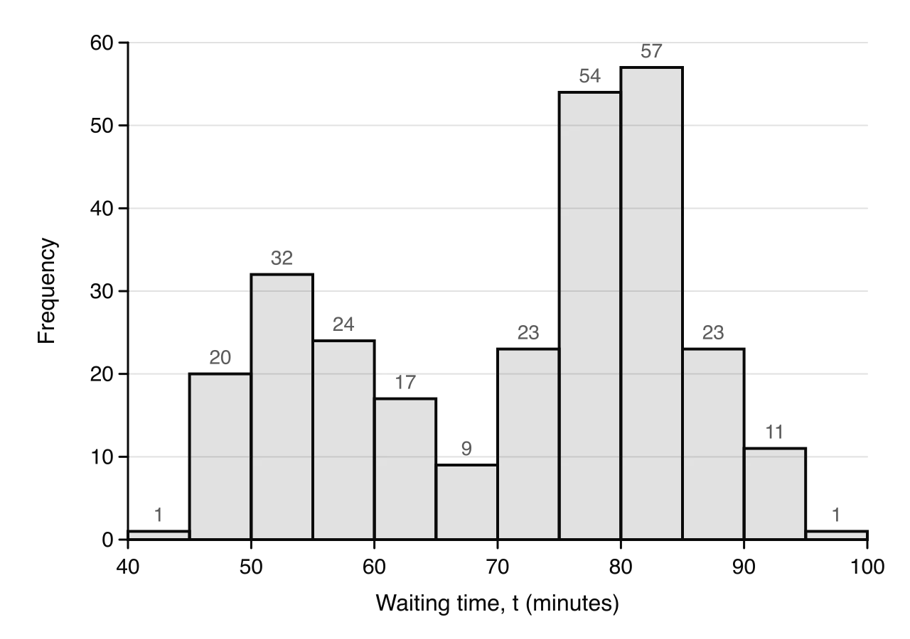
The waiting times form two clusters, one around 50–55 minutes and a larger one around 75–85 minutes. Data: Old Faithful geyser, 272 eruptions (Härdle, 1991).
The Old Faithful histogram shows a feature that the table hides: the waiting times form two separate groups. A distribution with two peaks is called bimodal. Geologists link the two groups to the length of the previous eruption: a short eruption is usually followed by a short wait, and a long eruption by a long wait.
Discrete data are shown in a bar chart (or vertical line graph) instead, with a separate bar or line at each value and gaps between them, because no values lie in between.
Reading a histogram
The class with the tallest bar is the modal class (see 4.3). The number of values in a range of classes is the sum of their frequencies. The overall shape (one peak or two, symmetric or with a long tail) is described in the last part of this subtopic.
Cumulative frequency
Cumulative frequency tables
The cumulative frequency up to a value is the number of data values less than or equal to it (for grouped data, less than the upper class boundary). It is a running total of the frequencies.
For the Old Faithful data, each cumulative frequency is the previous one plus the frequency of the next class.
Waiting time, t (minutes)
Cumulative frequency
t<45
1
t<50
21
t<55
53
t<60
77
t<65
94
t<70
103
t<75
126
t<80
180
t<85
237
t<90
260
t<95
271
t<100
272
The last cumulative frequency always equals the total number of data values, which is a useful check.
Cumulative frequency graphs
A cumulative frequency graph plots each cumulative frequency against the upper class boundary of its class, because only at the end of a class is it certain that all the values in it have been counted. The graph starts at the lower boundary of the first class with cumulative frequency 0. The points are joined with a smooth curve or with straight line segments; joining them with straight segments assumes the values are spread evenly within each class.
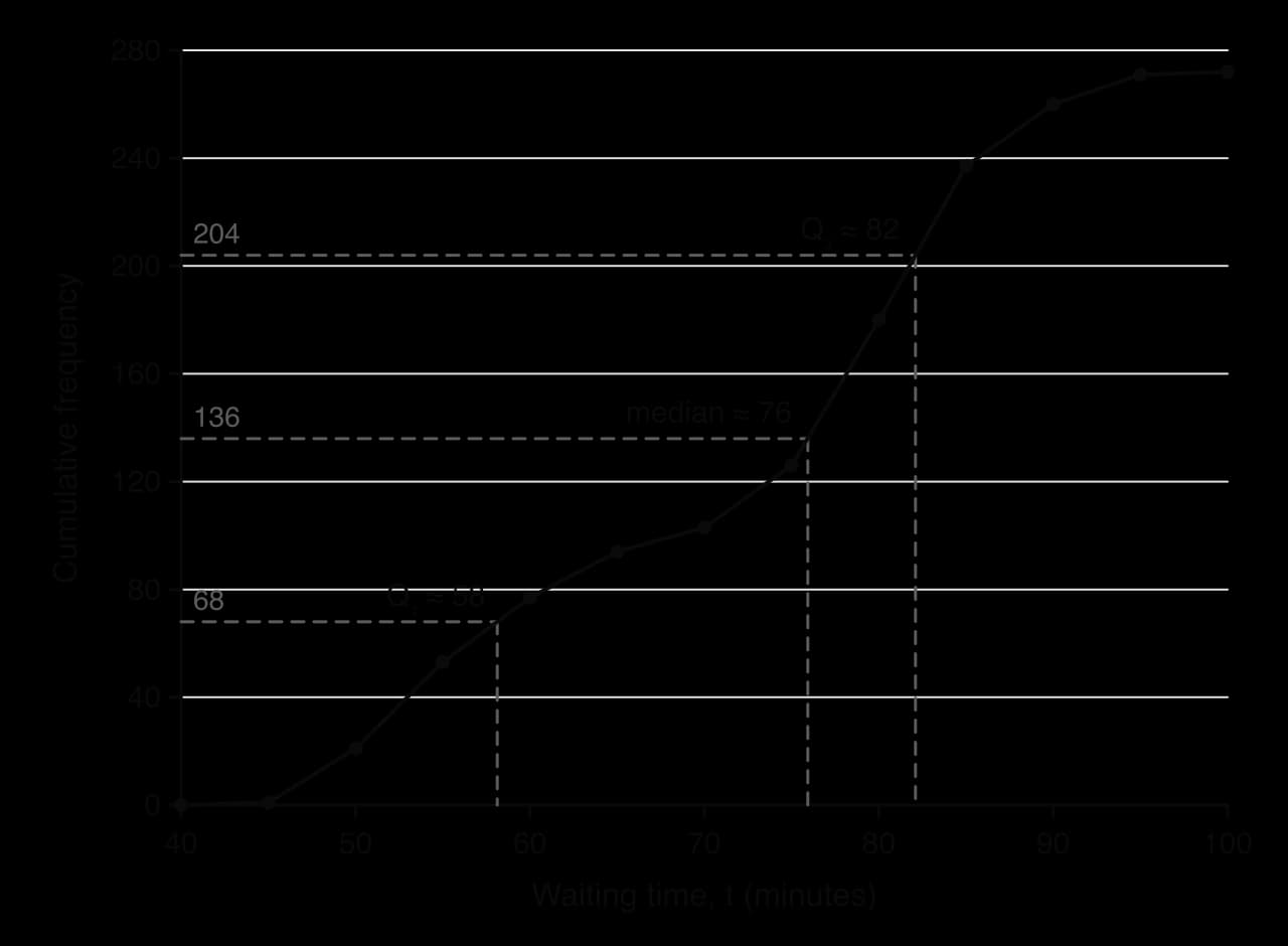
Read across from a quarter, a half and three quarters of 272, then down: Q₁ ≈ 58, median ≈ 76, Q₃ ≈ 82 minutes. The steepest part of the curve is where the data are most concentrated.
The gradient of the graph shows how densely the data are packed: the curve is steep where many values fall in a short interval (75 to 85 minutes) and nearly flat where there are few (65 to 70 minutes). A cumulative frequency graph is always increasing or level, never decreasing.
Median, quartiles and percentiles
Ordered data are divided into four equal parts by three values. The median is the middle value. The lower quartile Q1 has a quarter of the data below it, and the upper quartile Q3 has three quarters below it.
More generally, a percentile gives the value below which a stated percentage of the data lie. The 10th percentile has 10% of the data below it; Q1, the median and Q3 are the 25th, 50th and 75th percentiles.
To estimate any of these from a cumulative frequency graph with total frequency n:
Find the cumulative frequency: 4n for Q1, 2n for the median, 43n for Q3, and 100p×n for the pth percentile.
Draw a horizontal line from this value on the vertical axis to the curve.
Draw a vertical line down to the horizontal axis and read off the value.
For grouped data the values are estimates, because the exact data values are not known. The precise positions used for raw data, such as the 2n+1th value, matter only for small data sets; for a graph, use 2n, 4n and 43n.
Range and interquartile range
Two measures of spread can be found from the graph. The range is the largest value minus the smallest; from grouped data it can only be estimated, as the upper boundary of the last class minus the lower boundary of the first. The interquartile range is the spread of the middle half of the data.
The IQR is not affected by a few extreme values, because it ignores the lowest and highest quarters of the data. The range depends only on the two most extreme values, so a single outlier can change it a great deal.
These estimates agree well with the exact values from the raw data (Q1=58, median 76, Q3=82), because 272 values are spread fairly evenly within each class.
Reading the graph the other way
A cumulative frequency graph can also be read from the horizontal axis upwards. Starting at a value of the variable, go up to the curve and across to read how many data values lie below it. Dividing by n and multiplying by 100 gives the percentage of the data below that value, which is the percentile it represents.
Box-and-whisker diagrams
The five-number summary
A data set can be summarised by five values: the minimum, Q1, the median, Q3 and the maximum. A box-and-whisker diagram (box plot) draws this five-number summary to scale.
For raw data, the quartiles used in this course follow the method of a GDC (see 4.3 for the details): order the data, find the median, then take Q1 as the median of the values below it and Q3 as the median of the values above it, leaving out the median itself when the number of values is odd.
Outliers on a box plot
An outlier is a value more than 1.5×IQR beyond the nearer quartile. The two boundaries, sometimes called fences, are
Q1−1.5×IQRandQ3+1.5×IQR
Any value below the lower boundary or above the upper boundary is an outlier. On the box plot the whisker stops at the most extreme value that is not an outlier, and each outlier is marked separately with a cross. The boundaries themselves are not drawn.
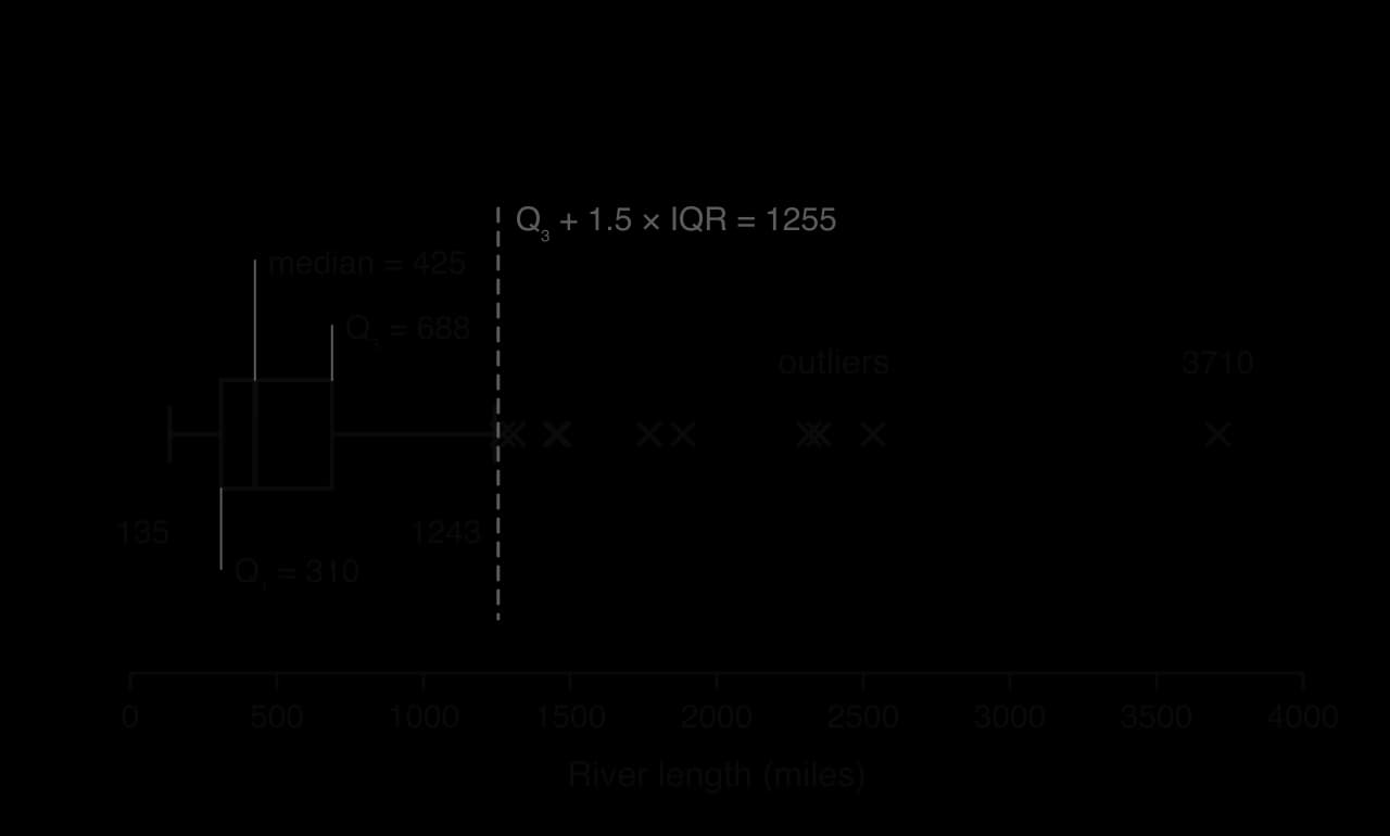
The upper whisker stops at 1243, the longest river within the boundary of 1255 miles; the ten longer rivers are plotted as outliers. Data: 141 major North American rivers, The World Almanac and Book of Facts (1975).
For the river lengths, IQR=688−310=378 miles, so the upper boundary is 688+1.5×378=1255 miles and the lower boundary is 310−567=−257 miles. No river can be shorter than −257 miles, so there are no low outliers, while ten rivers are longer than 1255 miles. Whether such values should be kept is discussed in 4.1: these are genuine rivers, so they stay.
Shape and skewness
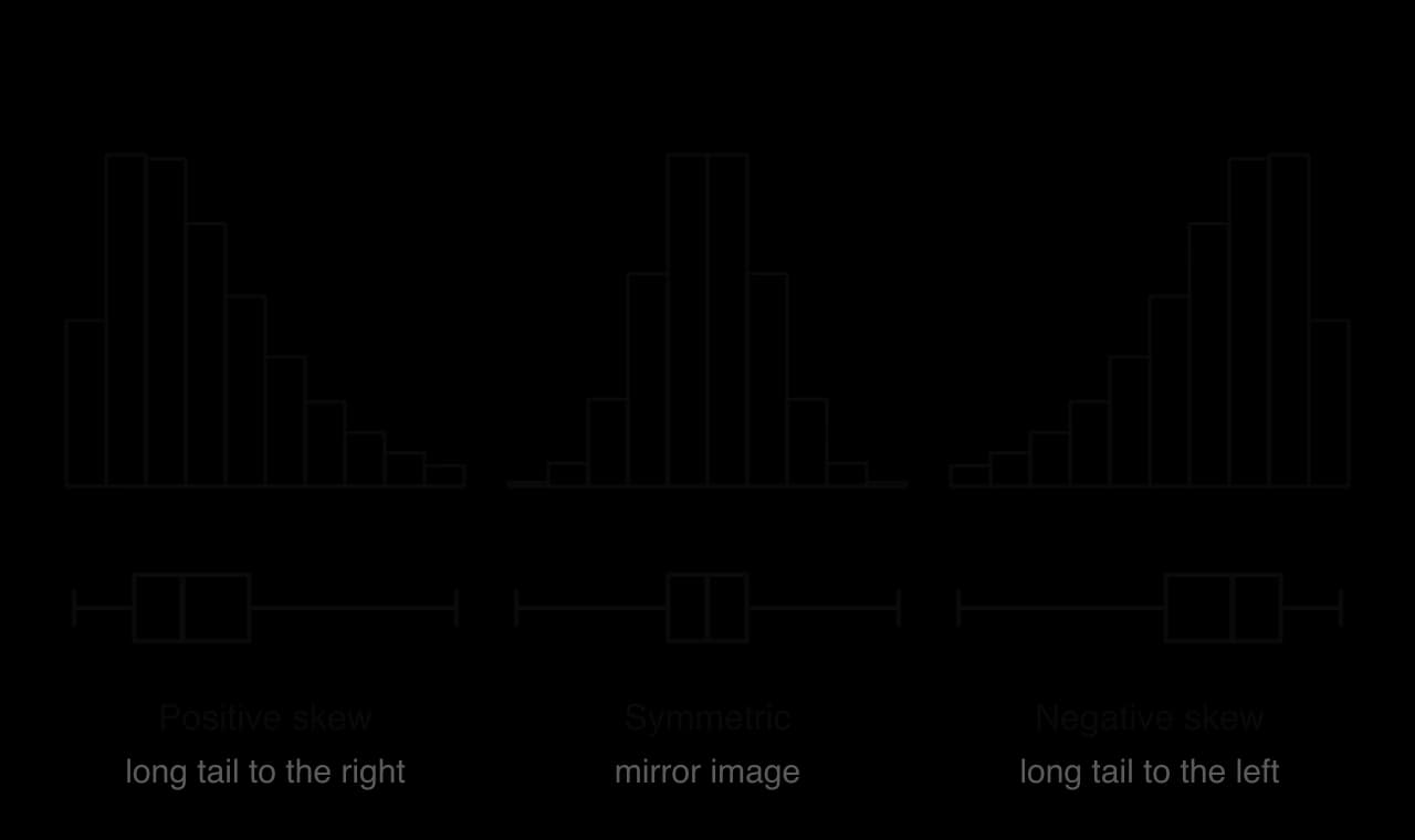
The shape of a distribution is described by its skewness. A symmetric distribution looks the same on both sides of its centre. A positively skewed distribution has a long tail to the right: most values are small, with a few much larger ones, as with incomes or the river lengths. A negatively skewed distribution has a long tail to the left: most values are large, with a few much smaller ones, as with the scores on an easy test.
The tail of the histogram and the longer whisker of the box plot point the same way. Positive skew: tail to the right; negative skew: tail to the left.
On a box plot, skewness shows in the position of the median within the box and in the lengths of the whiskers:
Shape
Median in the box
Whiskers
Symmetric
In the middle: Q3−median≈median−Q1
About equal
Positive skew
Nearer Q1: Q3−median>median−Q1
Right whisker longer
Negative skew
Nearer Q3: Q3−median<median−Q1
Skewness in this course is described informally, in words; it is not calculated. A box plot cannot show a bimodal shape: the Old Faithful waiting times, with their two peaks, give an ordinary-looking box plot, which is why a histogram should be drawn as well when the shape matters.
Comparing distributions with box plots
Box plots drawn one above the other on the same scale make it easy to compare data sets. A comparison should cover two things, always in the context of the data:
Centre: compare the medians, and say which group has typically higher values.
Spread: compare the IQRs (and the ranges), and say which group is more variable or more consistent.
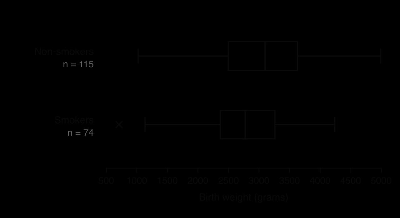
Shape and outliers can be mentioned as well. The parallel box plots compare the birth weights of babies whose mothers did or did not smoke during pregnancy.
The whole box for the smokers sits to the left of the non-smokers' box, and its median is about 325 g lower. Data: 189 births, Baystate Medical Center, Springfield, Massachusetts, 1986 (Hosmer and Lemeshow).
The data show an association between smoking and lower birth weight, but on their own they do not prove that smoking causes it, since mothers who smoked may differ in other ways. Correlation and causation are discussed in 4.4.
Proportions from a box plot
Because each section of a box plot (lower whisker, the two halves of the box, upper whisker) holds a quarter of the data, a box plot also shows proportions. About 25% of the values lie above Q3, 50% lie between Q1 and Q3, and so on. A value that falls between two of the five numbers can only be placed within a range of percentages.
Exam-style questions on presenting data
A race organiser recorded the times t minutes taken by 80 runners to complete a 5 km race, as summarised in the table.
Time, t (minutes)
Frequency
10≤t<15
4
15≤t<20
p
20≤t<25
25
25≤t<30
q
30≤t<35
8
35≤t<40
3
Self-check
To do:
I can construct frequency tables for discrete data and grouped frequency tables for continuous data.
To do:
I can find class boundaries, class widths and mid-interval values, including for rounded data and ages.
To do:
I can draw a histogram with equal class widths and describe the shape it shows.
To do:
I can construct a cumulative frequency table and graph, plotting at upper class boundaries.
To do:
I can estimate the median, quartiles, percentiles, range and IQR from a cumulative frequency graph.
To do:
I can find a five-number summary, identify outliers with the 1.5×IQR rule and draw a box plot.
To do:
I can describe a distribution as symmetric, positively skewed or negatively skewed.
To do:
I can compare two distributions from box plots, commenting on centre and spread in context.
below the lower quartile or more than
1.5×IQR
above the upper quartile.
(a)
Find the lower quartile and the upper quartile of the recorded heights.
[2]2 marks
Markscheme (a)
Q1=5.35A1
Q3=7.15A1
(b)
Show that 0.6 and 11.8 are both outliers.
[2]2 marks
Markscheme (b)
IQR=7.15−5.35=1.8(A1)
Q1−1.5×1.8=2.65
(c)
Every seedling was at least 3 cm tall when it was planted at the start of the three weeks. For each of the two outliers, state whether it should be kept in or removed from the data, giving a reason.
[2]2 marks
Markscheme (c)
0.6 should be removed: a seedling at least 3 cm tall cannot have a height of 0.6 cm three weeks later, so it must be an error in recording (e.g. a misplaced decimal point or a value in different units) R1
11.8 should be kept: it is possible for one seedling to grow much more than the others, so it is a valid (genuine) data value R1
Note: Award R1 for each correct decision with a valid reason. Do not award R1 for a decision without a reason.
Question 2 · AA-0039115 marks
A city council wants to find out about the journey times of the 18 000 people who travel into the city to work each weekday. An officer asks 120 people waiting at the central bus station between 08:00 and 08:30 on one Monday how long their journey to work takes.
(a)
Write down the name of the sampling method used by the officer.
[1]1 mark
(b)
Give two reasons why this sample may not be representative of all the people who travel into the city to work.
[2]2 marks
(c)(i)
The journey times, t minutes, of the 120 people are summarised in the following table.
Journey time, t minutes
Frequency
0≤t<10
9
10≤t<20
21
20≤t<30
34
30≤t<40
28
40≤t<50
17
50≤t<60
8
60≤t<70
3
Find an estimate of the mean and an estimate of the standard deviation of the journey times.
[3]3 marks
(c)(ii)
Write down the class interval that contains the median journey time.
[1]1 mark
(c)(iii)
One of these 120 people is chosen at random. Find the probability that their journey time is at least 40 minutes.
[1]1 mark
(d)(i)
The officer also kept the exact journey times. For these 120 values, the lower quartile is 21 minutes and the upper quartile is 39 minutes. An outlier is a value more than 1.5×IQR above the upper quartile or below the lower quartile.
Find the least journey time that would be an outlier.
[2]2 marks
(d)(ii)
The longest journey time in the sample is 68 minutes. State, with a reason, whether this value should be removed from the data.
[2]2 marks
(e)(i)
The following week, the council takes a systematic sample of 150 people from a list of the 15 000 people who hold a monthly travel pass for the city.
Find the sampling interval.
[2]2 marks
(e)(ii)
Explain why this sample may still not represent all the people who travel into the city to work.
A conservation team catches 200 fish from a lake using nets and measures the length of each fish, in cm. The lengths are summarised in the following table.
Minimum
Lower quartile
Median
Upper quartile
Maximum
9
18
23
27
52
An outlier is a value more than 1.5×IQR below the lower quartile or above the upper quartile.
(a)
State whether the length of a fish is a discrete or a continuous variable.
[1]1 mark
(b)
Show that the longest fish is an outlier, and that the shortest fish is not.
[3]3 marks
(c)
The longest fish was photographed when it was measured, and it is of a species that is known to grow to more than 60 cm. State, with a reason, whether its length should be kept in the data.
[1]1 mark
(d)
Estimate the number of these 200 fish that are shorter than 27 cm.
[2]2 marks
(e)
The holes in the nets let fish shorter than about 8 cm escape. Explain how this affects the use of these 200 fish to estimate the median length of all the fish in the lake.
[1]1 mark
(f)
The 200 fish are made up of 120 perch, 50 roach and 30 pike. A stratified sample of 40 of these fish, proportional to species, is chosen for further study. Find the number of fish of each species in this sample.
[2]2 marks
(g)
All 200 fish are tagged and returned to the lake. One month later, 150 fish are caught at random from the lake and 12 of them are found to be tagged. Assume that this second catch is a random sample of all the fish in the lake. Estimate the total number of fish in the lake.
[3]3 marks
(h)
State one further assumption needed for the estimate in part (g) to be reliable.
The upper half is 19,20,21,22,24,25,38, so Q3=22.
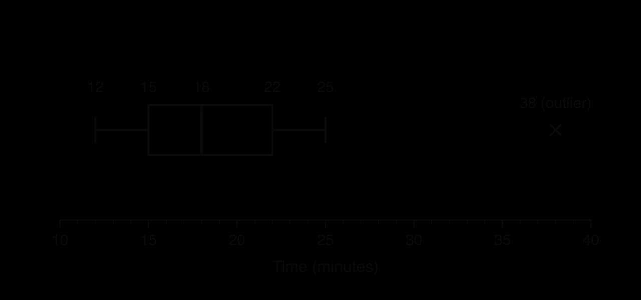
Five-number summary: minimum 12, Q1=15, median 18, Q3=22, maximum 38.
(b) IQR=22−15=7 and 1.5×7=10.5.
Q1−10.5=4.5Q3+10.5=32.5
Since 38>32.5, the value 38 is an outlier. Every other value lies between 4.5 and 32.5, so there are no other outliers.
(c) The upper whisker ends at 25, the largest value that is not an outlier, and 38 is marked with a cross.
The whisker ends at 25, not at 38, because 38 is an outlier.
Left whisker longer
. The upper half of the box is much longer than the lower half, and the right whisker (from 45 to 140) is far longer than the left (from 21 to 28). The distribution is positively skewed: most salaries are fairly low, with a long tail of high salaries.