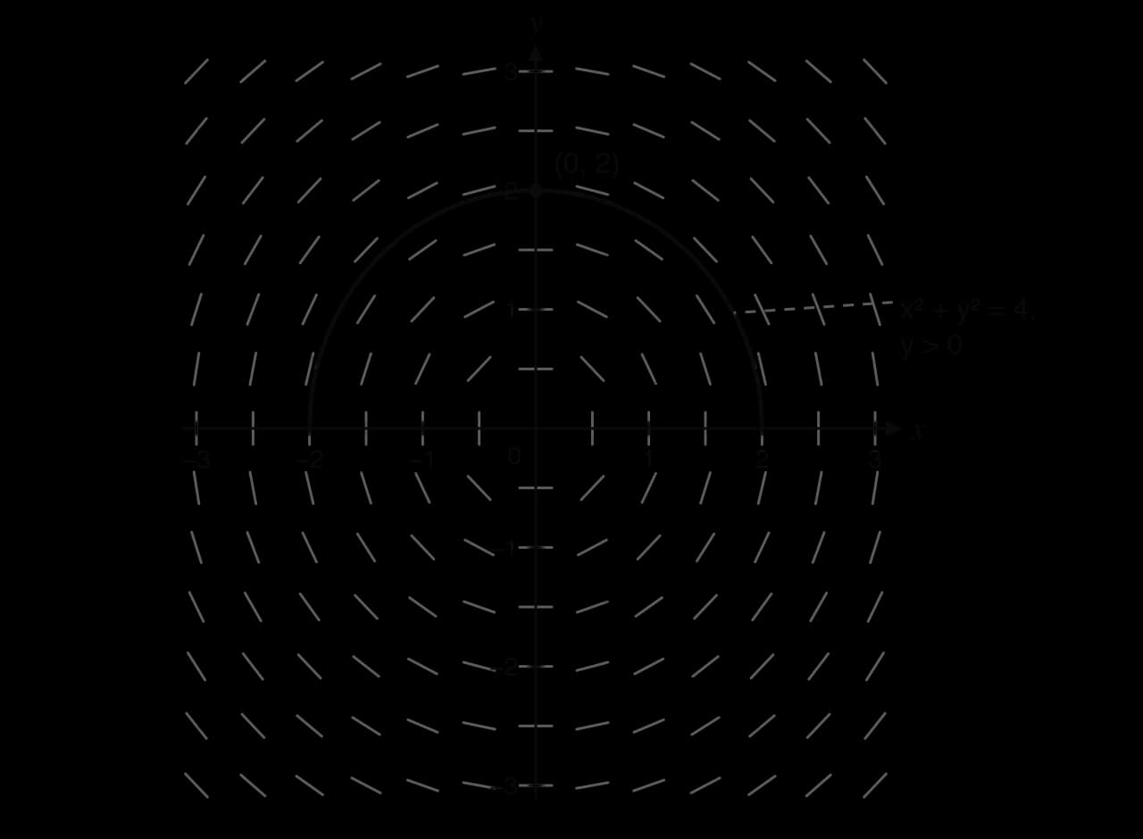
5.18 First-order differential equations

A differential equation describes how a quantity changes rather than what the quantity is. Many laws of science are stated this way: a population grows at a rate proportional to its size, a hot drink cools at a rate proportional to how much hotter it is than the room, and salt leaves a tank at a rate that depends on how much salt the tank holds. Solving the differential equation turns the rule for the rate of change into a formula for the quantity itself.

First-order differential equations bring together almost every integration technique in the course. They also give a different view of a function: a curve can be described by the gradient it must have at every point, and that description alone is enough to draw it, approximate it numerically or, for several important types of equation, find it exactly.

Differential equations and their solutions

What a differential equation is

An equation such as $y = x^2 + 3$ gives $y$ directly in terms of $x$. A differential equation instead gives information about the derivative of $y$, and the task is to work back to $y$

Examples of first-order differential equations include $\frac{dy}{dx} = 6x^2 - 4$, $\frac{dy}{dx} = 2y$

The simplest first-order equations have a right-hand side that depends on $x$ only. An equation of the form $\frac{dy}{dx} = f(x)$ is solved by integrating once, $y = \int f(x)\,dx$

The variables do not have to be $x$ and $y$. In models the independent variable is usually time $t$, and the dependent variable is named after what it measures: $P$ for a population, $T$ for a temperature, $S$ for a mass of salt. The equation $\frac{dP}{dt} = 0.03P$

Checking a solution

A function is a solution of a differential equation if substituting it, and its derivative, into the equation makes both sides identical for every value of $x$ in its domain. Checking a proposed solution needs only differentiation, so it is a useful first step before learning any method of solution.

"Show that" means every step towards the given result must be written down. Here that means differentiating, substituting into the right-hand side, and stating clearly that the two sides agree.

General and particular solutions

The example shows that one differential equation can have infinitely many solutions, one for each value of $C$. This mirrors the constant of integration in an indefinite integral: integrating loses the information about where the curve starts.

Each value of $C$ gives one solution curve. The curves fill the plane without crossing, and the initial condition picks out the one curve that passes through a chosen point. For $\frac{dy}{dx} = x - y$ with $y(0) = 1$

Slope fields

Drawing a slope field

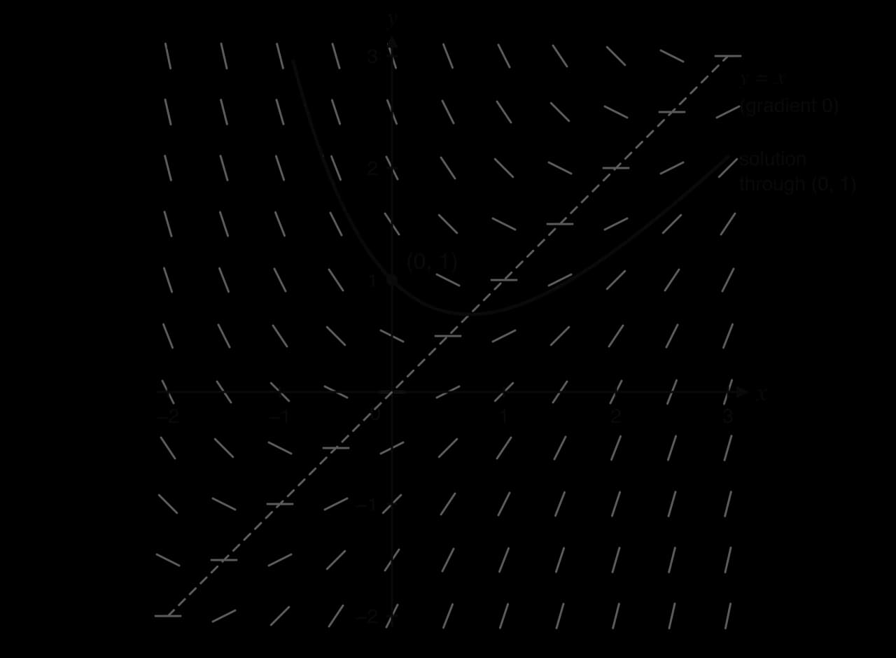
The equation $\frac{dy}{dx} = f(x, y)$ gives the gradient of the solution curve through every point $(x, y)$

For $\frac{dy}{dx} = x - y$, the gradient at $(2, 1)$ is $2 - 1 = 1$

Sketching solution curves

A solution curve follows the slope field: at every point it is tangent to the segment there. To sketch the solution through a given point, start at that point and move a little way in the direction of the nearby segments, then repeat, in both directions. The curve should run parallel to the segments it passes, never cut across them.

The curves through different points do not cross. If two solution curves met at a point, they would have the same gradient $f(x, y)$ there and would continue together, so for the equations in this course each point lies on exactly one solution curve.

Isoclines

Plotting a slope field point by point is slow. It is quicker to find the curves on which the gradient takes a fixed value.

For $\frac{dy}{dx} = x - y$, the isoclines $x - y = k$

Reading a slope field

Some features of the equation can be read straight from the field.

Euler's method

Small steps along the gradient

Many differential equations, such as $\frac{dy}{dx} = \sqrt{x + y}$

Starting at a known point $(x_0, y_0)$, the gradient there is $f(x_0, y_0)$

The formula is the tangent line approximation from differentiation, $\Delta y \approx \frac{dy}{dx} \times \Delta x$, applied once per step. The Euler estimates form a polygon of straight segments that tries to follow the true curve.

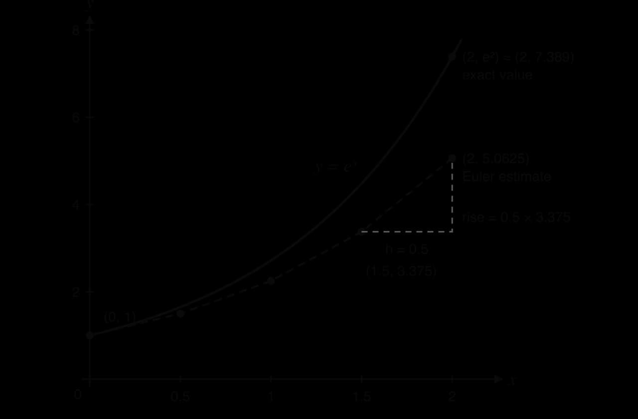
For $\frac{dy}{dx} = y$ with $y(0) = 1$, the exact solution is $y = e^x$

Setting out Euler's method

The calculation is clearest in a table with one row per step. Work with the unrounded values throughout and round only the final answer.

Euler's method on a GDC or spreadsheet

For more than a few steps, a graphic display calculator (GDC) or a spreadsheet does the repetition. On a spreadsheet, put $x_0$ and $y_0$ in the first row; each new row adds $h$ to the previous $x$ and computes $y + h \times f(x, y)$

The effect of the step length

Each Euler step follows a tangent, and the error made in one step depends on how far the curve bends away from its tangent over a distance $h$. Reducing $h$ reduces the error in each step, at the cost of needing more steps. For the equation $\frac{dy}{dx} = x - y$

Halving the step length roughly halves the error, and dividing it by 10 divides the error by about 10. The error is approximately proportional to $h$, so Euler's method improves steadily but slowly. More accurate numerical methods exist and are used by GDCs and software, but they rest on the same idea of building the curve from its gradient.

The sign of the error depends on the concavity of the solution curve. A curve that is concave up lies above its tangents, so Euler's method underestimates. A curve that is concave down lies below its tangents, so Euler's method overestimates. The concavity can be found from the differential equation itself: for $\frac{dy}{dx} = x - y$, differentiating gives $\frac{d^2y}{dx^2} = 1 - \frac{dy}{dx} = 1 - (x - y)$

Separation of variables

The method

A differential equation is separable when the right-hand side can be written as a function of $x$ multiplied by a function of $y$:

Dividing by $h(y)$ and writing $g(y) = \frac{1}{h(y)}$ gives $g(y)\frac{dy}{dx} = f(x)$

By the chain rule (or the substitution rule of 5.16), the left-hand side is $\int g(y)\,dy$. The equation becomes

with everything involving $y$ on one side and everything involving $x$ on the other.

The steps are:

1. Rearrange so that all of $y$ (with $dy$) is on one side and all of $x$ (with $dx$) is on the other.

2. Integrate both sides, writing one constant $C$ on the $x$

One constant is enough: constants on both sides, $G(y) + C_1 = F(x) + C_2$, combine into a single constant $C = C_2 - C_1$

Exponential growth and decay

The most important separable equation states that a quantity changes at a rate proportional to its size:

Separating, $\int \frac{1}{y}\,dy = \int k\,dx$, so $\ln|y| = kx + C$

Since $e^C$ is any positive constant and $y$ may be positive or negative, the two cases combine as $y = Ae^{kx}$, where $A = \pm e^C$

This explains why exponential functions model so many processes (2.9): any quantity whose rate of change is proportional to its current size must change exponentially.

Further separable equations

Separable equations can lead to any of the standard integrals, including those of 5.15 (HL). The right-hand side often has to be factorised or split, using laws of exponents, before the variables can be separated.

The next equation does not look separable until the exponential is split with the law $e^{a - b} = \frac{e^a}{e^b}$

Homogeneous differential equations

Recognising a homogeneous equation

Some equations that are not separable become separable after a change of variable. An important class has a right-hand side that depends only on the ratio $\frac{y}{x}$.

For example, $\frac{dy}{dx} = \frac{x^2 + y^2}{xy}$

The substitution y = vx

Writing $v = \frac{y}{x}$, so that $y = vx$ with $v$

The differential equation becomes

which is separable in $v$ and $x$:

After integrating, replace $v$ by $\frac{y}{x}$ to return to the original variables.

The integral in $v$ sometimes needs partial fractions (1.11), as in the next example.

Linear differential equations and the integrating factor

The standard form

A large class of equations that are neither separable nor homogeneous can be solved by a different method.

"Linear" refers to $y$: both $y$ and $\frac{dy}{dx}$ appear only to the first power and are never multiplied together or placed inside another function. The equations $\frac{dy}{dx} + y = x$

Why the integrating factor works

The left-hand side $\frac{dy}{dx} + P(x)y$ resembles the result of the product rule. The idea is to multiply the whole equation by a function $I(x)$ chosen so that the left-hand side becomes exactly the derivative of the product $yI$

The two sides match if $\frac{dI}{dx} = PI$. This is a separable equation for $I$, with solution $\ln I = \int P(x)\,dx$

Any one such function works, so no constant of integration is needed in the exponent.

The method:

1. Write the equation in standard form, so that the coefficient of $\frac{dy}{dx}$ is $1$. Read off $P(x)$ and $Q(x)$

The expression $e^{\int P(x)\,dx}$ almost always simplifies, using $e^{\ln u} = u$ and $e^{k\ln u} = u^k$

The constant of integration must be added before dividing by the integrating factor. In the last example it becomes the term $Cx^2$, which is part of every solution; adding $C$ after the division gives $x^2\sin x + C$, which does not satisfy the differential equation.

The integral $\int Q(x)I(x)\,dx$ may need integration by parts (5.16). The next example solves, with an integrating factor, the equation whose slope field and family of solutions opened the subtopic.

Choosing a method

Some equations can be solved by more than one method. The equation $\frac{dy}{dx} = 2y$, for instance, is separable and also linear. Checking the forms in order saves time.

Modelling with differential equations

Forming a differential equation

A model is often stated in words. "The rate of change of $N$" is $\frac{dN}{dt}$, "is proportional to" introduces a constant $k$, and a decreasing quantity has a negative rate of change.

Every model rests on assumptions. Exponential growth assumes unlimited resources, so it cannot hold for long; the cooling model assumes the surroundings stay at a fixed temperature; mixing models assume the tank is stirred so that the concentration is the same throughout. Commenting on whether these assumptions are reasonable is part of interpreting a model.

Newton's law of cooling

A hot object in a cooler room loses heat faster when the temperature difference is larger. The simplest model states that the rate of cooling is proportional to this difference.

The equation is separable. With $T > T_s$,

so $T - T_s = Ae^{-kt}$. At $t = 0$, $A = T_0 - T_s$

The temperature difference decays exponentially, and $T$ approaches the room temperature $T_s$ without reaching it. The equation is also linear, so an integrating factor $e^{kt}$ gives the same result.

Logistic growth

Exponential growth cannot continue for ever: food, space or other resources run out. The logistic model adds a factor that slows growth as the population approaches a maximum.

When $P$ is small, the bracket is close to $1$ and $\frac{dP}{dt} \approx rP$: growth is nearly exponential. As $P$

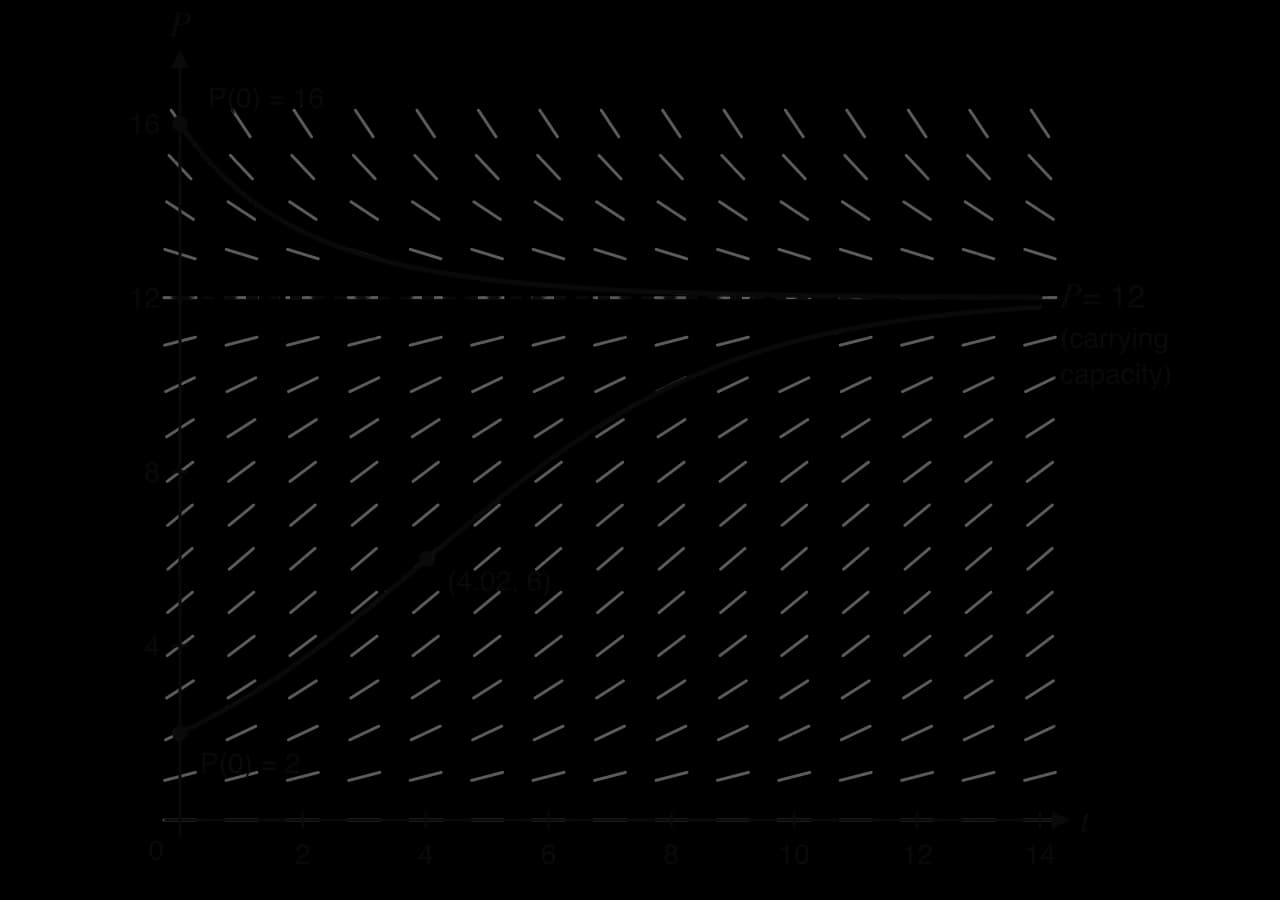
The growth rate $rP\left(1 - \frac{P}{K}\right)$ is a quadratic in $P$ with roots $0$

The logistic equation is separable. Using partial fractions,

Rewriting the equation as $\frac{K}{P(K - P)}\,dP = r\,dt$ and integrating, for $0 < P < K$

Solving for $P$ gives the logistic function

and $P_0 = P(0)$. As $t \to \infty$, $e^{-rt} \to 0$

Mixing problems

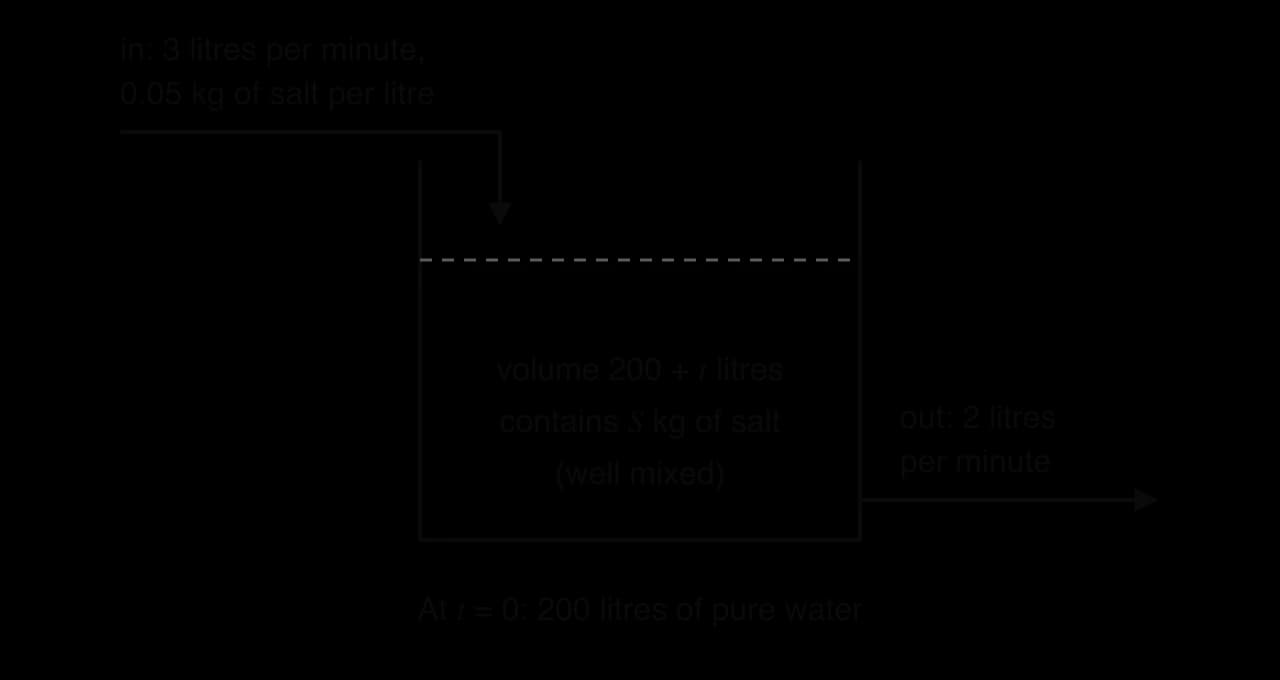
In a mixing problem a substance, such as salt, flows into and out of a tank of liquid. The amount of the substance changes at the rate it comes in minus the rate it goes out:

The rate in is the inflow rate multiplied by the concentration of the incoming liquid. Assuming the tank is well mixed, the rate out is the outflow rate multiplied by the concentration in the tank, $\frac{S}{V}$, where $V$ is the volume of liquid at that moment.

When the flows in and out are equal, the volume is constant. For a tank holding 200 litres of pure water, into which brine containing $0.05$ kg of salt per litre flows at 4 litres per minute while the mixture flows out at 4 litres per minute,

This is separable (or linear). Separating gives $\ln|0.2 - 0.02S| = -0.02t + c$, and with $S(0) = 0$ the solution is $S = 10\left(1 - e^{-0.02t}\right)$

When the flows differ, the volume changes and $V$ depends on $t$, which usually makes the equation linear but not separable.

Exam-style questions on differential equations

Differential equations often appear as long questions that combine a method of solution with Euler's method, a slope field or a model. The two questions that follow show typical structures; the first allows a GDC and the second does not.

Self-check

• To do:

  I can verify that a function satisfies a differential equation, and explain the difference between a general solution and a particular solution.

• To do:

  I can calculate gradients on a slope field, find isoclines and equilibrium solutions, and sketch a solution curve through a given point.

• To do:

  I can apply Euler's method by hand and with a GDC or spreadsheet, and explain how the step length and the concavity of the solution affect the error.

• To do:

  I can solve a separable differential equation, handling the constant of integration correctly when logarithms and exponentials are involved.

• To do:

  I can recognise a homogeneous equation and solve it with the substitution $y = vx$.

• To do:

  I can write a linear equation in standard form, find its integrating factor and solve it.

• To do:

  I can choose a suitable method for a given first-order differential equation.

• To do:

  I can form a differential equation from a description, solve it, and interpret the solution for exponential growth and decay, Newton's law of cooling, logistic growth and mixing.