2.5 Elasticity of demand · IB Economics | Augment Education
2.5 Elasticity of demand
Calculate and interpret price and income elasticities of demand, link PED to total revenue and tax revenue, draw the elasticity diagrams and the Engel curve, and evaluate how firms and governments use them.
IB Economics
Part of 2 Microeconomics
SL and HL
Key terms introduced here
Each is in the Economics glossary, with every other term in the subject.
The factors that decide how price elastic demand for a good is: the number and closeness of substitutes, the degree of necessity, the proportion of income spent on it, and time.
A measure of how responsive one economic variable is to a change in another, calculated as the percentage change in the first divided by the percentage change in the second.
Demand for which the percentage change in quantity demanded is larger than the percentage change in income, so that YED is greater than 1; typical of luxury goods and many services.
A measure of the responsiveness of the demand for a good to a change in consumers' income, ceteris paribus: the percentage change in quantity demanded divided by the percentage change in income.
Demand for which the percentage change in quantity demanded is smaller than the percentage change in income, so that YED lies between 0 and 1; typical of necessities.
Explain the concept of elasticity and draw relatively elastic and relatively inelastic demand curves.
Calculate price elasticity of demand (PED) and use it to find changes in price, quantity demanded and total revenue.
Explain the range of PED values and draw perfectly elastic, perfectly inelastic and unitary elastic demand curves.
Explain the determinants of PED and the relationship between PED and total revenue.
Evaluate the importance of PED for firms’ pricing decisions and for governments’ indirect taxes.
Explain why PED changes along a straight-line demand curve and why PED for primary commodities is lower than for manufactured products (HL).
Calculate income elasticity of demand (YED), interpret its sign and size, and draw an Engel curve.
Evaluate the importance of YED for firms and for changes in the sectoral structure of an economy (HL).
Introduction
The law of demand says that consumers buy less of a good when its price rises, but not how much less. Elasticity measures the size of that response, and the size decides what happens to a firm’s sales revenue after a price change, how much revenue a government raises from a tax, and which industries grow as a country becomes richer.
Elasticity connects several key concepts. Consumers facing scarcity make different choices when prices and incomes change; governments use elasticity to judge an intervention such as a tax on sugary drinks; and income elasticity helps to explain long-run change in the structure of whole economies.
Questions on 2.5
137 exam-style questions on this subtopic, written in the style of the IB papers. The first has its markscheme open. Counted on
Question 1 · ECON-000018 marks
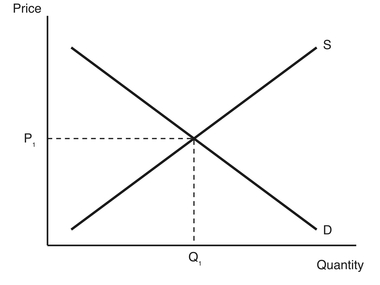
The diagram shows the market for bus tickets in a city, in equilibrium at price P1 and quantity Q1.
Try a quick-fire question
One of 56 short multiple-choice questions on 2.5. Pick an answer to see why it's right or wrong.
The diagram shows a rise in price from P₁ to P₂. If demand is price inelastic between P₁ and P₂, which statement must be true?
Flashcards for 2.5
The official deck for this part of the syllabus.
2.5 Elasticity of demand · front
What is elasticity in economics?
2.5 Elasticity of demand · front
Explain two reasons why elasticity is measured with percentage changes rather than absolute changes.
2.5 Elasticity of demand217 cards
Carry on with 2.5 in Augment
With a free account, Augment remembers where you stopped and what you have practiced.
The change in a variable expressed as a percentage of its original value: the new value minus the original value, divided by the original value, multiplied by 100.
Demand for which any rise in price above the current level causes quantity demanded to fall to zero, so that PED is infinite and the demand curve is horizontal.
Demand for which the percentage change in quantity demanded is larger than the percentage change in price, so that PED is greater than 1, ignoring the minus sign.
A measure of the responsiveness of the quantity demanded of a good to a change in its own price, ceteris paribus: the percentage change in quantity demanded divided by the percentage change in price.
Demand for which the percentage change in quantity demanded is smaller than the percentage change in price, so that PED lies between 0 and 1, ignoring the minus sign.
A raw material or agricultural product produced in the primary sector and traded with little or no processing, such as crude oil, copper, wheat or coffee.
A change in the shares of output and employment produced by the primary, secondary and tertiary sectors, usually from primary to secondary and then tertiary as incomes rise.
Demand for which the percentage change in quantity demanded equals the percentage change in price, so that PED is exactly 1 and total spending does not change when price changes.
Scope: At SL and HL, elasticity of demand includes the concept of elasticity, price elasticity of demand (its formula, values, determinants, link with total revenue and use by firms and governments) and income elasticity of demand (its formula, sign and size, and the Engel curve), with the related calculations. HL adds how PED changes along a straight-line demand curve, why PED for primary commodities is low, and why YED matters for firms and for sectoral change. Cross-price elasticity of demand is not part of the syllabus.
What elasticity measures
Many economic variables respond to changes in other variables. Quantity demanded responds to price, to income and to the prices of related goods; quantity supplied responds to price. Elasticity is a single number that says how strongly one variable responds to a change in another.
Elasticity is always calculated from percentage changes, not absolute changes. A rise of 1,000 units means a great deal in a market that sells 2,000 units and almost nothing in a market that sells 2 million. Percentages also make elasticity independent of units: the result is the same whether quantity is measured in litres or barrels and price in pesos or dollars, so elasticities can be compared across goods and countries.
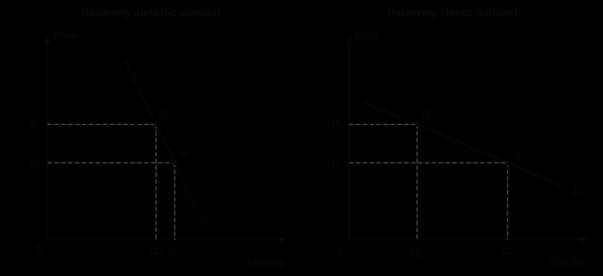
When the response is large, demand is described as elastic; when it is small, demand is inelastic. The two panels in the figure show the same rise in price, from P₁ to P₂, in two markets. On the steep curve the quantity demanded falls only slightly; on the flat curve it falls a lot.
The same price rise from P₁ to P₂ cuts quantity demanded only slightly when demand is relatively inelastic (left) and by much more when it is relatively elastic (right).
Comparing two curves drawn on the same axes and scale, the flatter one is the more elastic over the same price range. Elasticity is not the same thing as slope, however. Slope measures absolute changes (units of quantity per dollar), while elasticity measures percentage changes, and along most demand curves the two give different answers.
Price elasticity of demand (PED)
The most widely used elasticity, price elasticity of demand (PED), measures how the quantity of a good that consumers demand responds to a change in its own price, with all other influences on demand held constant (ceteris paribus).
PED=percentage change in pricepercentage change in quantity demanded
The percentage change in quantity demanded always goes on top, because quantity is the variable that responds. The calculation has three steps: work out the percentage change in quantity demanded, work out the percentage change in price, and divide the first by the second.
The same formula can be rearranged to find a missing value. If the PED and the percentage change in price are known, the percentage change in quantity demanded is PED × %ΔP. If the PED and the change in quantity are known, the change in price is %ΔQd ÷ PED.
%ΔQd=PED×%ΔP%ΔP=PED%ΔQd
The sign of PED
Because price and quantity demanded move in opposite directions (the law of demand), PED is almost always negative: a positive change in price comes with a negative change in quantity, and the other way round. Economists usually ignore the minus sign and compare the absolute value with 1, so a PED of −0.4 is described as “0.4” or “less than 1”. A good with a PED of −2 is more price elastic than one with a PED of −0.5, even though −2 is the smaller number.
The range of PED values
PED can take any absolute value from zero to infinity. Five categories are used to describe it, and each has its own name and diagram.
Price inelastic demand is typical of goods that consumers regard as necessities, that have few close substitutes or that take a small share of income: tap water, salt, petrol in the short run, cigarettes for a regular smoker.
Price elastic demand is typical of goods with many close substitutes, such as one brand of breakfast cereal or a particular airline on a busy route, and of goods that take a large share of income.
Two further cases are extremes that rarely exist for a whole market but are useful benchmarks, and the perfectly elastic case describes the demand facing a single small firm in a highly competitive market.
A patient who needs a fixed dose of a life-saving medicine, such as insulin, comes close to perfectly inelastic demand over a wide range of prices.
Three curves with the same PED all along them. Horizontal: PED is infinite. Vertical: PED is zero. Rectangular hyperbola: PED is 1, so spending P × Q is the same at every price (areas A and B are equal).
The third panel shows a unitary elastic demand curve. It is a curve, not a straight line, called a rectangular hyperbola: every point on it gives the same total spending, price × quantity. A 10% fall in price is met by an increase in quantity that leaves spending unchanged, so area A (P₁ × Q₁) equals area B (P₂ × Q₂). The table brings the five cases together.
PED (absolute value)
Description
Demand curve
Response of quantity to a 10% price rise
0
Perfectly inelastic
Vertical
No change
Between 0 and 1
Price inelastic
Relatively steep
Falls by less than 10%
1
Unitary elastic
Rectangular hyperbola
Falls by exactly 10%
Between 1 and ∞
Price elastic
Relatively flat
Falls by more than 10%
∞
Perfectly elastic
Horizontal
Falls to zero
Determinants of PED
Demand for petrol as a whole is price inelastic, while demand for one brand of petrol is price elastic. The determinants of PED explain the difference. Each of them works through the same idea: the easier it is for consumers to avoid a price rise, the more elastic their demand.
Number and closeness of substitutes
This is the most important determinant. When a good has many close substitutes, a rise in its price leads consumers to switch, so quantity demanded falls sharply and demand is price elastic. When there are few or no close substitutes, consumers keep buying and demand is price inelastic.
How closely a market is defined matters. Demand for “food” as a whole is very inelastic, because there is no substitute for eating. Demand for “bread” is more elastic, since rice and pasta can replace it, and demand for one supermarket’s own brand of bread is highly elastic because other brands sit on the next shelf. The narrower the definition, the more substitutes there are and the higher the PED.
Substitutes also exist in space. When Philadelphia added a tax of 1.5 cents per ounce to sweetened drinks in January 2017, the volume of taxed drinks sold by large chain stores in the city fell by about half, but sales in the bordering Pennsylvania areas rose by about 308 million ounces, offsetting roughly a quarter of the fall. For many shoppers, the same drinks sold a short drive away were a close substitute.
Sources: Roberto et al., _JAMA (2019)._
Degree of necessity
A necessity is something consumers feel they cannot do without, either because it meets a basic need (staple foods, heating, medicine) or because they are addicted to it (tobacco, alcohol for some drinkers). Demand for necessities is price inelastic. Goods that consumers regard as optional, such as restaurant meals, foreign holidays or designer clothing, have more elastic demand, because the purchase can easily be postponed or dropped.
Whether something is a necessity depends on the consumer. A regular smoker treats cigarettes as a necessity; a teenager who has just started smoking, with less income and a weaker habit, responds more to price. The World Health Organization describes tobacco taxes as the most cost-effective way to reduce tobacco use, especially among young people and low-income groups, which is what a higher PED in those groups predicts.
Sources: World Health Organization, “Tobacco” fact sheet (accessed October 2026).
Proportion of income spent on the good
When a good takes up a tiny share of a consumer’s income, such as a box of matches or a packet of salt, even a large percentage rise in its price makes little difference to the household budget, so demand is inelastic. When a good takes a large share of income, such as a car, rent or a holiday, a price rise forces a real cut in spending elsewhere, so consumers respond more and demand is more elastic.
The same good can take very different shares of income in different households. Food is a small share of spending in rich households and a large share in poor ones, so low-income consumers tend to respond more to food price changes.
Time
In the short run, consumers are often locked into their habits and their equipment. A commuter who drives a petrol car to work cannot change car, job or home the week the price of petrol jumps. Over a longer period, consumers can find substitutes: they buy more fuel-efficient or electric cars, move closer to work, or use public transport. Demand is therefore more price elastic in the long run than in the short run.
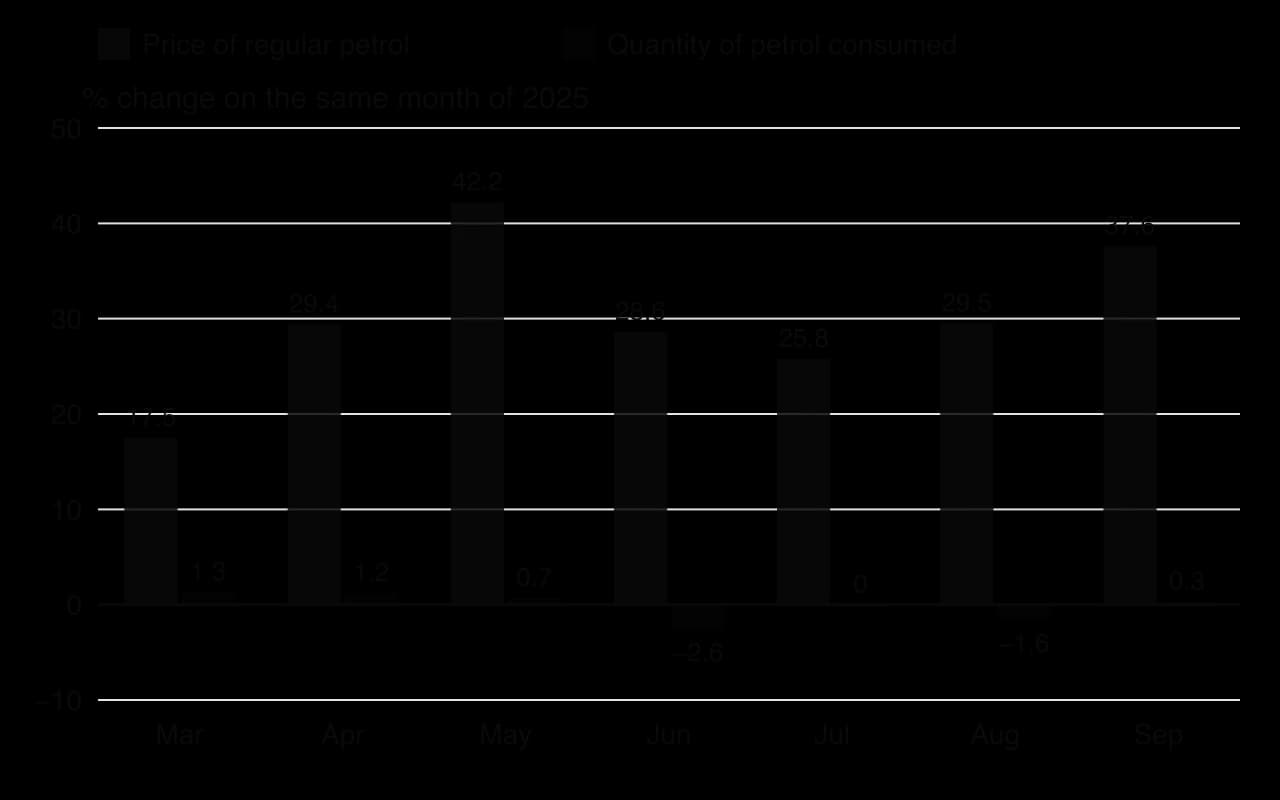
The 2026 oil shock shows the short-run case clearly. After shipping through the Strait of Hormuz was disrupted from late February 2026, the average US price of regular petrol was between 18% and 42% higher than a year earlier in every month from March to September, yet the quantity of petrol consumed stayed within about 3% of its level a year before.
US petrol prices rose by up to 42% on a year earlier in 2026, but the quantity consumed barely changed: in the short run demand for petrol is highly price inelastic. Source: US EIA, weekly product supplied, and FRED (GASREGW), October 2026.
The chart compares each month with the same month a year earlier, so other influences, such as rising incomes and population, also affect the quantity bars and the numbers cannot be read as an exact PED. The pattern, a large price change with almost no change in quantity, is still what a very low short-run PED predicts. If prices stay high, the long-run response should be larger as households replace their cars.
Determinant
Demand tends to be more price elastic when…
Demand tends to be more price inelastic when…
Substitutes
there are many close substitutes, or the market is narrowly defined (one brand)
there are few or no close substitutes, or the market is broadly defined (food)
Degree of necessity
the good is a luxury or can easily be postponed
the good meets a basic need or is habit-forming
Proportion of income
the good takes a large share of income
the good takes a tiny share of income
Time
consumers have had a long time to adjust
the price change is recent
YouTube
EconplusDal explains the PED formula, the range of values and the determinants of PED, with worked calculations.
PED and total revenue
A firm’s total revenue is the amount it receives from selling its output. It depends on both the price and the quantity sold, so a price change pulls revenue in two directions at once. PED decides which pull is stronger.
Total revenue is the same number as total consumer spending on the good, seen from the seller’s side. On a demand diagram it is the area of the rectangle under the demand curve from the origin up to the price and across to the quantity.
Why PED decides what happens to revenue
When a firm raises its price, it gains revenue on every unit it still sells, because each unit now brings in more. It also loses revenue on the units that consumers no longer buy. When demand is price inelastic, the fall in quantity is proportionally small, so the gain from the higher price outweighs the loss of sales and total revenue rises. When demand is price elastic, the fall in quantity is proportionally large, so the loss of sales outweighs the gain and total revenue falls.
After a price rise from P₁ to P₂, the firm gains area A and loses area B; C is kept. With inelastic demand A is bigger than B, so total revenue rises; with elastic demand B is bigger, so total revenue falls.
The diagram shows this as areas. Before the price rise, revenue is P₁ × Q₁, rectangles C + B. After it, revenue is P₂ × Q₂, rectangles C + A. Area A is the extra revenue from charging more on the units still sold; area B is the revenue lost on the units no longer bought. On the inelastic curve (left) A is clearly larger than B; on the elastic curve (right) B is larger than A.
PED
Price rise
Price cut
Inelastic (0 < PED < 1)
TR rises
TR falls
Unitary elastic (PED = 1)
TR unchanged
TR unchanged
Elastic (PED > 1)
TR falls
TR rises
In short, when demand is price inelastic, price and total revenue move in the same direction; when it is price elastic, they move in opposite directions. A firm that wants to raise its revenue should raise its price if demand is inelastic and cut it if demand is elastic.
Misjudging PED can be expensive. In July 2011 Netflix split its combined plan into separate streaming and DVD-rental plans at $7.99 a month each, which many customers saw as a price rise for using both. About 800,000 customers cancelled, and the company soon dropped its plan to separate the DVD business. With rival ways to watch films available, demand was more elastic than the firm expected.
Sources: Wikipedia, “Netflix” (accessed October 2026), from company announcements (2011).
Changing PED along a straight-line demand curve (HL only)
A straight-line demand curve has the same slope everywhere: every $1 fall in price raises quantity demanded by the same number of units. Its elasticity, however, falls steadily as the price falls, because the same absolute changes are different percentage changes at different points on the line.
At a high price, quantity demanded is small. A given increase in quantity is therefore a large percentage of a small number, while a $1 price cut is a small percentage of a high price. The ratio of the two percentages is large, so demand is price elastic. At a low price the opposite holds: the same increase in quantity is a small percentage of a large quantity, the same $1 price cut is a large percentage of a low price, and demand is price inelastic.
The PED formula can be rewritten to show this. The first term is the inverse of the slope, which is constant along a straight line; the second term, P/Q, falls continuously as the price falls and the quantity rises.
PED=%ΔP%ΔQd=ΔP/PΔQd/Q=ΔPΔQd×QP
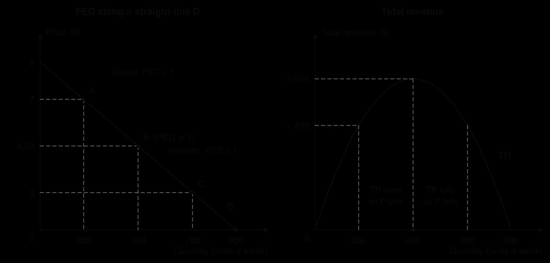
PED is above 1 on the upper half of the line (point A), exactly 1 at the midpoint B and below 1 on the lower half (point C). Total revenue is highest at the midpoint, where PED = 1.
The figure shows the result for a demand curve that meets the price axis at $9 and the quantity axis at 900 units a week. At the top of the line, where quantity is close to zero, PED tends to infinity. At the midpoint B, half of the maximum price, PED is exactly 1. Below the midpoint demand is inelastic, and where the line meets the quantity axis PED is zero. The right-hand panel links this to total revenue: cutting the price raises revenue as long as demand is elastic, revenue reaches its maximum at the unitary elastic midpoint, and further price cuts reduce revenue in the inelastic range.
Why PED matters for firms and governments
Knowing PED, even approximately, helps decision-makers predict the results of their choices. Firms use it when they set prices; governments use it when they choose which goods to tax and when they predict how a tax will change behaviour.
PED and firms’ pricing decisions
A firm that wants to increase its revenue raises prices on products with inelastic demand and cuts prices, or offers discounts, on products with elastic demand. This is why firms work hard to make demand for their products less elastic: advertising, brand loyalty, loyalty schemes and subscription contracts all reduce the number of goods consumers see as close substitutes, giving the firm more freedom to raise prices.
Firms also use differences in PED between groups of customers. Airlines charge high fares to business travellers, whose employers pay and who must travel on a given day (inelastic demand), and lower fares to holidaymakers, who can choose another date, airline or destination (elastic demand). Cinemas, museums and train operators charge students and pensioners less for the same reason.
PED also helps firms decide how to deal with rising costs. A firm facing inelastic demand can pass much of an increase in costs on to consumers with little loss of sales; a firm facing elastic demand must absorb more of it.
PED and governments: indirect taxes
An indirect tax is a tax on spending, such as a tax per litre of petrol or a percentage tax on the price of a good. PED decides two things about it: how much revenue it raises, and who bears the burden (tax incidence).
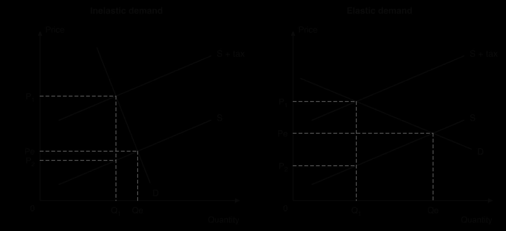
The same tax per unit shifts supply up by the tax. With inelastic demand, price rises most of the way to P₁, quantity barely falls and tax revenue (shaded) is large; with elastic demand, quantity falls a lot and revenue is smaller.
In the left-hand panel, demand is price inelastic. The tax shifts the supply curve vertically upwards by the tax per unit, from S to S + tax. Consumers keep buying, so quantity falls only slightly from Qe to Q₁, and the price consumers pay rises from Pe to P₁, which is most of the tax. Producers receive P₂, only slightly below Pe. The shaded rectangle, (P₁ − P₂) × Q₁, which is the tax per unit multiplied by the quantity sold, is the government’s revenue, and it is large because the quantity taxed hardly falls.
In the right-hand panel, demand is price elastic. The price consumers pay rises only a little, producers absorb more of the tax, and quantity falls a long way, so the tax raises less revenue. These are the two lessons for governments. Taxes on goods with inelastic demand raise a lot of revenue and fall mostly on consumers; taxes on goods with elastic demand raise less and fall more on producers.
This creates a tension when a government taxes a demerit good such as cigarettes or sugary drinks. If the aim is to raise revenue, inelastic demand is helpful. If the aim is to cut consumption, inelastic demand works against the tax: a large tax may be needed for a small fall in quantity. Taxes on goods with very inelastic demand also tend to take a larger share of the income of poorer households, which raises questions of equity.
Evaluating PED as a guide to decisions
PED is useful, but decision-makers rarely know its true value. Estimates come from past data, in which many other things changed at the same time as price, so the ceteris paribus condition is never fully met. A single estimate may also hide large differences between groups of consumers, regions or time periods.
PED also changes over time and with circumstances. Demand that is inelastic in the short run can become much more elastic in the long run, as the petrol example shows, so a tax that raises a lot of revenue in its first year may raise less later. For a firm, rivals may respond to a price change: a price cut that would raise revenue if competitors kept their prices may not if they cut theirs too, because PED estimates usually assume other prices stay the same.
Strengths of using PED
Limitations of using PED
Predicts the direction of the change in total revenue after a price change
Estimates are based on past data and may be out of date
Helps governments forecast tax revenue and the effect of a tax on consumption
Ceteris paribus rarely holds: incomes, tastes and rivals’ prices change too
Shows who bears the burden of a tax (consumers or producers)
PED differs between groups, places and time periods
Explains why firms advertise and build brand loyalty
Short-run and long-run PED can differ greatly
The table summarises how elasticity links to the key concepts.
Key concept
How elasticity applies
Choice
PED and YED describe how consumers change their choices when prices and incomes change.
Intervention
PED decides how much revenue a tax raises and how far it reduces consumption.
Equity
Taxes on goods with inelastic demand, such as food and fuel, can fall heavily on low-income households.
Change
Demand becomes more elastic over time, and YED explains how spending patterns change as incomes rise.
PED for primary commodities and manufactured products (HL only)
Most primary commodities are traded in large international markets at prices set by world demand and supply, and many low- and middle-income countries earn most of their export revenue from one or two of them.
Demand for primary commodities is generally price inelastic, for reasons that follow directly from the determinants of PED.
Necessity. Many commodities are basic needs (staple foods such as wheat and rice) or essential inputs without which production stops (crude oil, natural gas, copper for electrical wiring).
Few substitutes. There is no close substitute for oil in most transport, or for wheat in bread, at least in the short run. Commodities are also standardised: one tonne of copper is much like another, so buyers switch between suppliers, not away from the commodity itself.
Small share of the final price. Many commodities are inputs whose cost is only a small part of the price of the final product. A rise in the price of cocoa beans changes the price of a chocolate bar by a small percentage, so manufacturers keep buying cocoa.
Time. Machinery, power stations and vehicles are built to use particular commodities, so users cannot change them quickly when prices rise.
Manufactured products usually face more elastic demand. Most are sold in markets with many competing brands and models, they are often not necessities, and buyers can postpone purchases of durable goods such as cars, televisions and furniture when prices rise.
Low PED for commodities matters because, combined with low price elasticity of supply, it means that small shifts in demand or supply cause large swings in commodity prices. This commodity price volatility creates serious problems for countries that depend on commodity exports.
Income elasticity of demand (YED)
Price is not the only influence on demand. When incomes rise, consumers buy more of some goods, about the same of others and less of a few. Income elasticity of demand measures this response.
YED=percentage change in incomepercentage change in quantity demanded
A change in income shifts the whole demand curve, so YED measures how far demand shifts at a given price. Unlike PED, the sign of YED carries information and must never be ignored.
The sign of YED: normal and inferior goods
For a normal good, demand rises when income rises, so YED is positive. Most goods and services are normal goods. For an inferior good, demand falls when income rises, because consumers switch to better alternatives they can now afford, so YED is negative. Examples include bus travel in many cities (replaced by cars and taxis), the cheapest own-brand foods and second-hand clothing.
The size of YED: necessities, luxuries and services
Among normal goods, the size of YED shows whether spending on the good grows faster or slower than income.
Goods with income inelastic demand are necessities: basic food, water, electricity, toothpaste. As income rises, consumers buy somewhat more of them, but spending on them rises more slowly than income, so they take a falling share of the household budget.
Which goods count as necessities depends on income. For a very poor household, rice or cooking oil may take most of the budget and behave like a luxury; for a middle-income household the same goods are necessities, bought in roughly the same amounts whatever happens to income.
Goods and services with income elastic demand are luxury goods and many services: foreign holidays, restaurant meals, private education, financial services, entertainment. As income rises, spending on them rises faster than income, so they take a growing share of the budget.
YED
Type of good
When income rises by 10%, quantity demanded…
Examples
Negative (< 0)
Inferior good
falls
Bus travel, cheapest own-brand foods
Between 0 and 1
Normal good: necessity (income inelastic)
rises by less than 10%
Staple foods, electricity, water
Greater than 1
Normal good: luxury or service (income elastic)
rises by more than 10%
Foreign holidays, restaurant meals
As with PED, the formula can be rearranged. If YED is 0.6 and incomes rise by 10%, quantity demanded rises by 0.6 × 10% = 6%. If YED is 1.8 and demand has risen by 9%, income must have risen by 9% ÷ 1.8 = 5%.
The Engel curve
The relationship between income and the quantity demanded of a good can be drawn as an Engel curve, named after the 19th-century statistician Ernst Engel, who found that poorer families spend a larger share of their income on food.
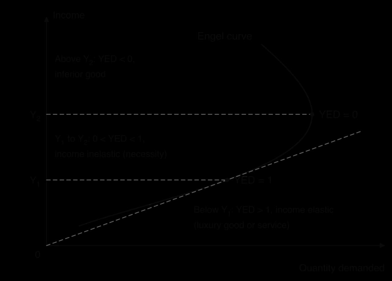
As income rises, the same good can move from income elastic (below Y₁), to income inelastic (Y₁ to Y₂), to inferior (above Y₂), where the curve bends back and demand falls as income rises further.
Income is drawn on the vertical axis and quantity demanded on the horizontal axis. Where the curve slopes upwards, the good is normal; where it bends backwards, so that higher income goes with a lower quantity, the good is inferior. The dashed line from the origin helps to read YED: where the Engel curve is flatter than a straight line from the origin to that point, quantity is growing proportionally faster than income and YED is above 1; where it is steeper, YED is between 0 and 1.
The figure follows one good through rising income. A low-income household treats it as a luxury (YED > 1), a middle-income household as a necessity (0 < YED < 1), and a high-income household replaces it with something better (YED < 0). Many foods follow this path: for a very poor household, meat or packaged rice is a luxury; as income rises it becomes a staple; at high incomes the cheapest versions are replaced by better ones.
YouTube
EconplusDal on income elasticity of demand: normal and inferior goods, necessities and luxuries, with calculations. The part on cross-price elasticity can be skipped.
Why YED matters (HL only)
YED and firms
Firms use YED to plan output and investment. In an economy whose incomes are rising, firms that sell goods with high YED (cars, holidays, luxury goods, financial services) can expect demand to grow faster than the economy, so they expand capacity and hire. Firms selling goods with low YED can expect slow growth in demand.
YED also tells firms how exposed they are to the business cycle. In a recession, when incomes fall, demand for income elastic goods falls sharply, while demand for necessities holds up and demand for inferior goods may even rise. Discount supermarkets and second-hand retailers often gain customers in recessions, while luxury brands and restaurants lose them.
Firms therefore use YED to choose a range of products that spreads this risk. A supermarket chain that sells both premium and budget own-brand ranges can shift its shelf space and promotions as incomes rise and fall. A car maker may add smaller, cheaper models to its range to protect sales in a downturn.
YED estimates have the same limits as PED estimates: they are based on past data, they differ between income groups and countries, and a good can move from luxury to necessity as it becomes common, as mobile phones did. Firms use them as one input to planning, alongside forecasts of how incomes themselves will change.
YED and the sectoral structure of the economy
YED also explains one of the most important long-run patterns in economic development: as countries grow richer, production and employment move from agriculture (the primary sector) to industry (the secondary sector) and then to services (the tertiary sector).
Its output is mostly primary commodities, and in low-income economies it often employs the largest share of the workforce.
Its output ranges from processed foods and clothing to cars, electronics and buildings.
Food and other agricultural products are necessities with low YED. As incomes rise, spending on them grows much more slowly than income, so the share of income spent on primary products falls. Manufactured goods and, above all, services such as health care, education, travel and entertainment have higher YED, so their share of spending rises. Firms respond to these shifts in demand, and labour and capital move out of the primary sector into the secondary and tertiary sectors. This process is sectoral change.
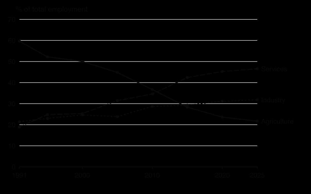
As incomes in China rose, agriculture’s share of jobs fell from 60% to 22% and services rose from 19% to 47%. Source: ILO modelled estimates via World Bank, World Development Indicators (2026).
China shows the pattern clearly. In 1991 almost 60% of its workers were in agriculture and fewer than one in five in services. By 2025 agriculture employed about 22% of workers, industry about 32% and services about 47%. Rising incomes moved demand towards manufactured goods and services, and workers followed it from farms to factories and offices.
YED is only part of the explanation. Productivity growth in agriculture frees workers to move to other sectors; trade lets countries specialise in manufactured exports even when domestic demand is still mostly for food; and government policy, such as China’s promotion of export industries, speeds or slows the process. For a commodity-exporting country, the low YED of its exports means that its export revenue grows slowly as world incomes rise, which is one reason governments try to diversify their economies.
Case study: Mexico’s tax on sugary drinks
In 2011 Mexicans drank more soft drinks per person than people in any other country, about 163 litres a year, and around 70% of adults were overweight or obese. From 1 January 2014 the federal government applied an excise tax of 1 peso per litre to non-dairy, non-alcoholic drinks with added sugar, which researchers estimated at about a 10% rise in price at 2013 prices. Prices rose by about the full amount of the tax from the first month, so the tax was passed on to consumers almost completely.
Researchers compared the drinks actually bought by more than 6,000 urban households with the amount predicted from the trend before the tax. The results show a response that was moderate at first and grew over time.
Measure (compared with the pre-tax trend)
Change in purchases of taxed drinks
Implied PED (price rise ≈ 10%)
Average over 2014
−6%
≈ −0.6
December 2014
−12%
≈ −1.2
Low-income households, average over 2014
−9%
≈ −0.9
Average over 2015
−9.7%
≈ −1.0
Untaxed drinks (mainly bottled water), 2014
+4%
—
Sources: Colchero et al., _BMJ (2016); Colchero et al., Health Affairs (2017)._
What the evidence shows about PED
Dividing the change in purchases by the roughly 10% rise in price gives an estimate of PED. Over 2014 as a whole it was about −0.6, so demand was price inelastic and the tax cut purchases by less, proportionally, than it raised the price. By December 2014, though, purchases were 12% below trend, implying a PED of about −1.2, and the fall in 2015 was larger than in 2014. This is the time determinant at work: consumers changed their habits gradually, and the response grew as they did.
Substitutes also mattered. Purchases of untaxed drinks rose by 4% in 2014, mainly bottled plain water, which is a close substitute for the purpose of quenching thirst. The response was largest among households of low socioeconomic status, for whom sugary drinks took a larger share of income. All four determinants of PED (substitutes, necessity and habit, share of income and time) appear in the results.
Revenue, health and equity
The tax shows the tension between the two aims of an indirect tax. Because demand was inelastic in the short run, most of the tax was paid by consumers and the government collected substantial revenue, but the fall in consumption was moderate. A larger tax, or more time, would be needed for a larger health effect. Mexico’s senate resolved to use part of the revenue to provide drinking water in schools, which would itself make demand for sugary drinks more elastic by making a substitute easier to find.
The tax also raises a question of equity. Low-income households paid a larger share of their income in tax, which makes the tax regressive in the short run. Supporters argue that the same households also cut consumption the most, so they gain most of the health benefit, and that spending the revenue on them could offset the burden.
Limits of the evidence
The estimates compare actual purchases with a prediction based on past trends, so they depend on that prediction being right. The data cover purchases in stores by urban households, not drinks consumed in restaurants or street stalls or in rural areas, and the price rise of about 10% is an average across very different drinks and pack sizes. A later study using national household surveys found a smaller fall of about 4% in purchases of taxed drinks over the four years after the tax. The direction of the effect is consistent across studies; its exact size, and so the exact PED, is less certain.
Sources: Colchero et al., _BMJ 352:h6704 (2016); Colchero et al., Health Affairs 36(3) (2017); García-Chávez et al., BMJ Public Health (2025)._
Exam practice
Elasticity appears in every paper. Paper 2 often asks you to define PED or YED, to calculate an elasticity or a change in revenue from data in the text, and to draw a diagram such as the PED and total revenue diagram. Paper 1 asks you to explain and evaluate the uses of PED, often in questions on indirect taxes. HL Paper 3 adds calculations from straight-line demand curves.
Paper 2 also asks for diagrams. A typical item is: “Using an appropriate diagram, explain why a rise in the price of electricity may increase the revenue of electricity suppliers [4].” Draw a steep demand curve, show the price rise from P₁ to P₂ and the small fall in quantity from Q₁ to Q₂, label the revenue gained and lost, and explain that demand is inelastic because electricity is a necessity with few substitutes, so the gain from the higher price outweighs the loss from lower sales.
Part (b) usually builds on the theory of part (a) but adds evaluation and real-world examples, so the same diagram can be reused with new analysis.
HL Paper 3 tests the same ideas with straight-line demand curves and asks for exact values.
Summary
Elasticity measures how responsive one variable is to a change in another, using percentage changes.
PED = %ΔQd ÷ %ΔP. It is negative; its absolute value classifies demand as perfectly inelastic (0), inelastic (0–1), unitary elastic (1), elastic (above 1) or perfectly elastic (∞).
PED depends on the number and closeness of substitutes, the degree of necessity, the share of income spent on the good, and time.
When demand is inelastic, price and total revenue move in the same direction; when it is elastic, they move in opposite directions.
Taxes on goods with inelastic demand raise more revenue and fall mainly on consumers, but cut consumption less.
HL: PED falls along a straight-line demand curve from elastic to inelastic; demand for primary commodities is less elastic than for manufactured products.
YED = %ΔQd ÷ %ΔY: negative for inferior goods, between 0 and 1 for necessities, above 1 for luxuries and many services; the Engel curve shows the relationship.
HL: YED helps firms plan output over the business cycle and explains the shift from primary to secondary and tertiary sectors as incomes rise.
Self-check
To do:
I can define elasticity and PED, and draw relatively elastic and relatively inelastic demand curves.
To do:
I can calculate PED from data, and use PED to find a change in quantity demanded, price or total revenue.
To do:
I can describe the range of PED values and draw perfectly elastic, perfectly inelastic and unitary elastic demand curves.
To do:
I can explain the four determinants of PED using a specific good.
To do:
I can draw and explain the diagram linking PED to changes in total revenue.
To do:
I can evaluate the use of PED by firms and governments, including for indirect taxes.
To do:
I can explain why PED changes along a straight-line demand curve and why PED for primary commodities is low (HL).
To do:
I can calculate YED, interpret its sign and size, and draw an Engel curve.
To do:
I can evaluate the importance of YED for firms and for sectoral change (HL).
The market for bus tickets.
When the bus company raised the ticket price from $2.00 to $2.50, the number of tickets sold per day fell from 40 000 to 36 000.
(a)
Define price elasticity of demand.
[2]2 marks
Markscheme (a)
A measure of the responsiveness of quantity demanded to a change in price, ceteris paribus. 2
Award 1 mark for a vague or partial definition.
(b)
Calculate the price elasticity of demand for bus tickets.
[2]2 marks
Markscheme (b)
%ΔQd=−10%, %ΔP=25%1
PED=25−10=−0.41
(c)
Using your answer to (b), explain the effect of the price rise on the bus company’s total revenue.
[4]4 marks
Markscheme (c)
Demand is price inelastic (|PED| < 1). 1
The percentage fall in quantity is smaller than the percentage rise in price. 1
Total revenue rises from $80 000 to $90 000 per day. 2
Question 2 · ECON-0009825 marks
Economists use simplified models to predict how markets will respond to changes in government policy.
(a)
Explain the role of economic models and the ceteris paribus assumption in predicting the effect of an indirect tax on a market.
[10]10 marks
(b)
Using real-world examples, evaluate the importance of price elasticity of demand (PED) for governments when deciding which goods to tax.
Read the extract and answer the questions that follow.
Text A — Testing the effect of Cerulia's sugar levy
[1] In January 2024 Cerulia introduced a levy on soft drinks containing more than 8 g of sugar per 100 ml. Before the levy was introduced, health economists at the national university put forward the hypothesis that demand for sugary soft drinks is price inelastic, so the levy would raise substantial revenue but reduce consumption only slightly.
[2] After the levy, the average price of a 1.5-litre bottle of sugary soft drink rose from 2.00 cerulian lira (CRL) to CRL 2.30. Monthly sales of sugary soft drinks fell from 18.0 million bottles to 16.2 million bottles.
[3] The researchers noted that over the same period a national advertising campaign warned about the health risks of sugar, and several manufacturers launched new low-sugar versions of their drinks.
(a)
Define the term hypothesis indicated in bold in the text (Text A, paragraph 1).
[2]2 marks
(b)(i)
Using information from Text A, paragraph 2, calculate the price elasticity of demand (PED) for sugary soft drinks in Cerulia.
[2]2 marks
(b)(ii)
Using your answer to (b)(i), state whether the evidence supports or refutes the economists' hypothesis.
[1]1 mark
(c)
Using a demand and supply diagram, explain the effect of the levy on the market for sugary soft drinks in Cerulia (Text A, paragraph 2).
[4]4 marks
(d)
Using information from Text A, paragraph 3, explain two reasons why the PED calculated in (b)(i) may not accurately measure the responsiveness of demand to the levy.