2.6 Elasticity of supply

Supply for which the percentage change in quantity supplied is smaller than the percentage change in price, so that PES lies between 0 and 1.

What price elasticity of supply measures

The law of supply says that firms offer more for sale when the price of their product rises, ceteris paribus, because a higher price makes extra output profitable. PES measures how strong that response is. It applies the same idea of elasticity used for demand to the supply side of the market.

Because price and quantity supplied normally move in the same direction, both percentage changes have the same sign and PES is positive. Unlike PED, there is no minus sign to ignore. A PES above 1 means that the quantity supplied changes proportionally more than price; a PES below 1 means it changes proportionally less.

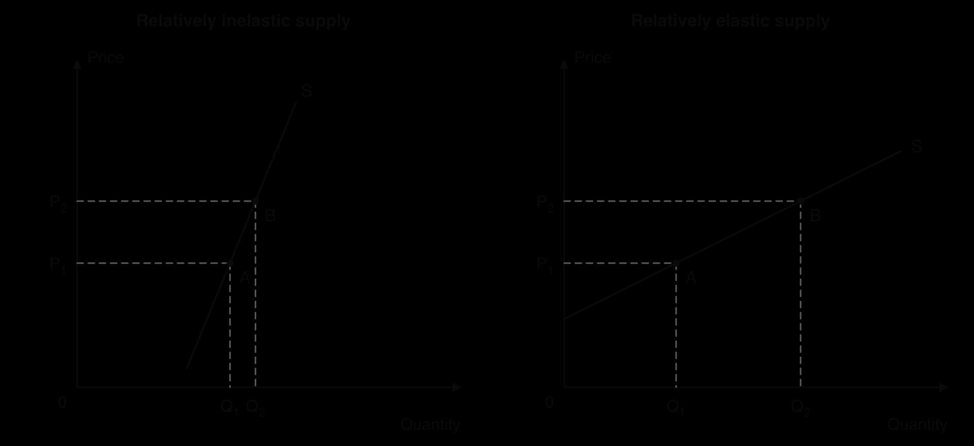
The figure shows the same rise in price in two markets. On the left, the supply curve is steep: producers can only add a little output, so quantity supplied rises from Q₁ to Q₂ by a small amount. On the right, the supply curve is flat: producers can expand output easily, and quantity supplied rises a lot.

The formula can be rearranged in the same way as the PED formula. The percentage change in quantity supplied is PES × %ΔP, and the percentage change in price needed for a given change in output is %ΔQs ÷ PES.

The range of PES values

Like PED, PES can take any value from zero to infinity, and the same five categories are used to describe it.

Price inelastic supply is typical where output takes a long time to increase, such as farm crops within a growing season, new housing or electricity generation.

Price elastic supply is typical of manufactured goods made in factories with spare machines and workers, and of goods held in large stocks.

Two extreme cases complete the range. Perfectly inelastic supply describes a fixed quantity, such as the seats in a stadium on match day or original paintings by an artist who has died. Perfectly elastic supply describes a market in which producers will supply any quantity at the going price but nothing below it; it is approached when many firms can produce a standard good at the same constant cost.

A vertical supply curve means that a rise in demand changes only the price, never the quantity. Tickets for a concert in a hall with a fixed number of seats are a standard example.

A horizontal supply curve means that a rise in demand changes only the quantity, never the price. It describes, approximately, the supply of a standard manufactured good, such as plain paper or screws, made by many firms that can all expand output at the same cost per unit. A small country that buys a good on the world market at the world price also faces supply that is close to perfectly elastic, because its purchases are too small to affect that price.

Why every straight line through the origin has a PES of 1

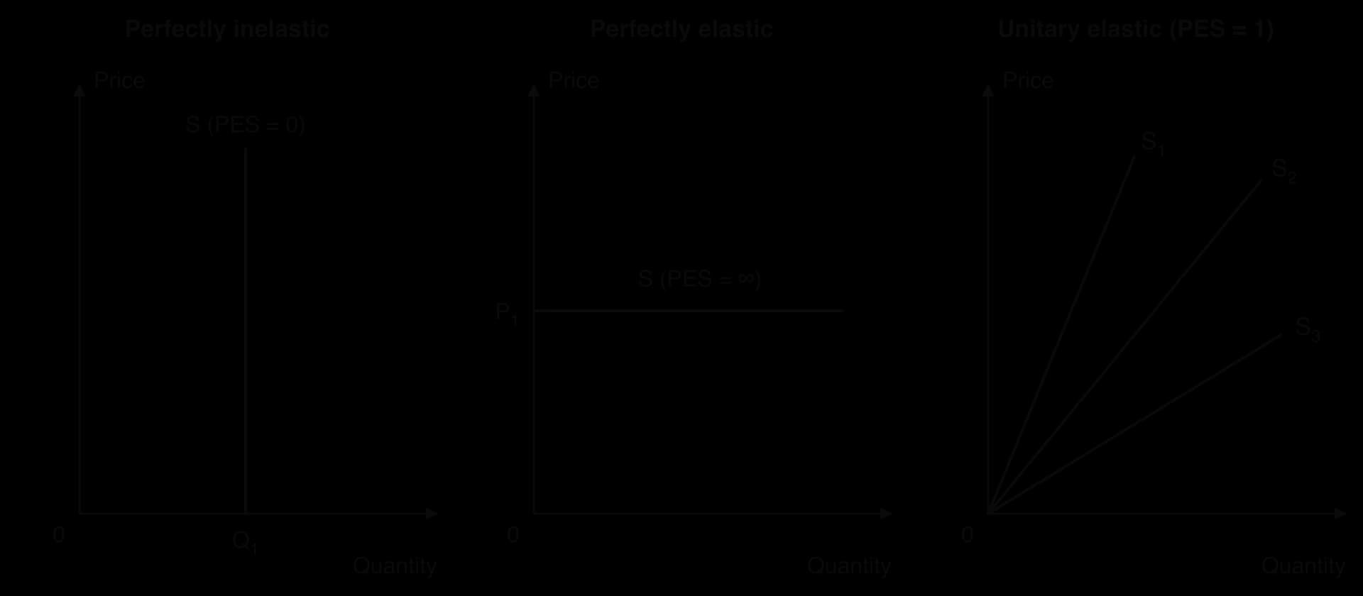
The third panel of the figure shows three supply curves of very different slopes, and all of them have the same PES. Along a straight line through the origin, quantity is always the same multiple of price. If the price doubles, the quantity doubles; if the price rises by 10%, the quantity rises by 10%. The slope only sets how many units are supplied per dollar, not the proportional response.

The table reads two points off each of two lines through the origin (hypothetical values). On the steep line, ten times fewer units are supplied at each price than on the flat line, but in both cases doubling the price doubles the quantity, so PES is 1 on both.

The same reasoning gives a quick rule for any straight supply curve. If it starts on the price axis (it cuts the vertical axis above the origin), supply is price elastic at every point, PES > 1. If it starts on the quantity axis (it cuts the horizontal axis to the right of the origin), supply is price inelastic at every point, PES < 1. Only lines through the origin are unitary elastic.

Determinants of PES

Whether a firm can increase output quickly when the price rises depends on how easily it can find extra inputs and how fast it can turn them into output. Five determinants decide this.

Time

Time is the most important determinant of PES. Economists distinguish three periods, which are defined by what producers can change, not by a fixed number of weeks or months.

• The momentary period: output cannot be changed at all, because the goods for sale are already produced. A fishing boat that has landed its catch can only sell what is in the hold. Supply is perfectly inelastic.

• The short run: firms can change their variable inputs, such as labour, raw materials and hours worked, but not their fixed inputs, such as land, buildings and machines. Output can rise a little, by running existing factories longer or hiring more workers, so supply is inelastic or moderately elastic.

• The long run: all inputs can be changed. Firms can build new factories, plant new land and train new workers, and new firms can enter the market. Supply is much more elastic.

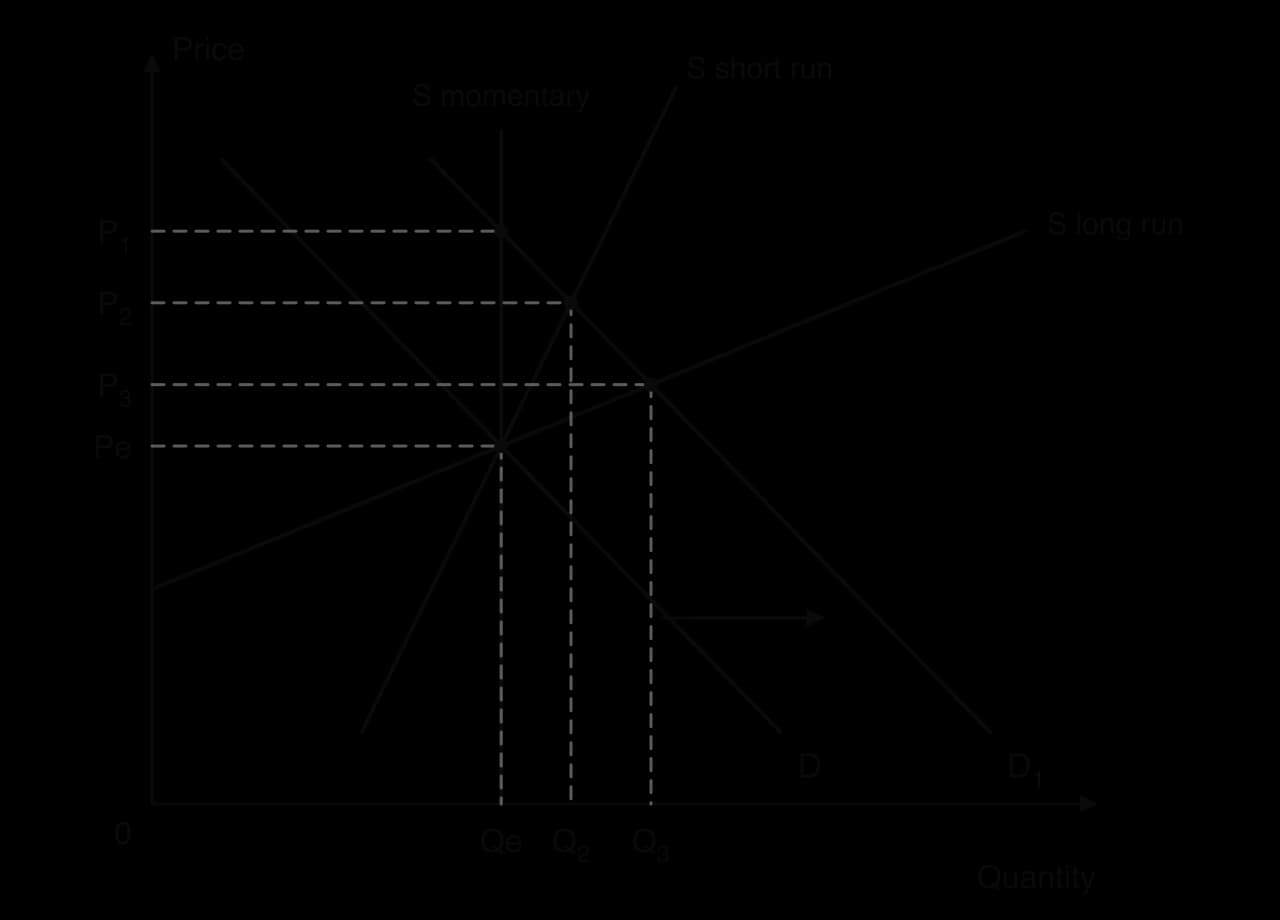
The diagram follows a rise in demand from D to D₁ through the three periods. With a fixed quantity, the whole adjustment falls on the price, which rises from Pe to P₁. In the short run, firms expand output along the steeper short-run supply curve, so price falls back to P₂ and quantity rises to Q₂. In the long run, new capacity and new firms make supply more elastic; the price settles at P₃, only a little above Pe, and the quantity rises to Q₃.

How long the short run lasts depends on the industry. Christmas trees take years to grow: Douglas firs are typically ready for sale only after five to seven years, so the number of trees available in a given December is almost fixed. Advanced semiconductors take years to bring to market too. TSMC announced its first chip factory in Phoenix, Arizona, in 2020; volume production began only in early 2025.

Sources: Wikipedia, “Christmas tree cultivation” and “TSMC Arizona” (accessed October 2026).

Energy markets showed the same constraint in 2021–2022. When Russian pipeline gas to Europe fell, European buyers turned to imported liquefied natural gas, but export terminals, tankers and import terminals take years to build. The price of natural gas in Europe rose from an average of $3.24 per million British thermal units in 2020 to $70.04 in August 2022. With supply so inelastic in the short run, the price had to rise far enough to cut the quantity demanded instead.

Sources: World Bank, Commodity Price Data (Pink Sheet), October 2026.

Mobility of factors of production

Firms can expand output quickly when the factors of production they need can be moved easily from other uses. Workers with general skills, standard machines and buildings that can be used for many purposes are mobile; specialised equipment, skilled professionals who take years to train and land suited to one crop are not.

The greater the mobility of factors of production, the more elastic supply is. In 2020, when demand for face masks rose suddenly, firms in other industries converted production lines to make them; the electronics arm of the Chinese carmaker BYD was one of the firms making masks that year. Supply of masks became elastic once these factors had been switched. Supply of doctors, by contrast, is inelastic for many years, because training them takes most of a decade.

Spare capacity

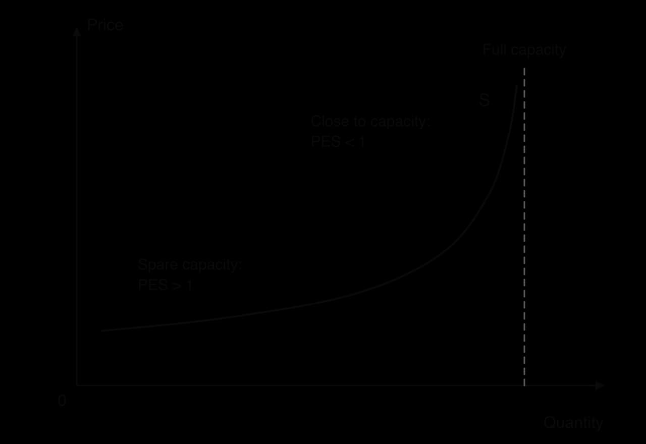
A firm with spare capacity has machines, buildings and workers that are not fully used. It can raise output quickly and at little extra cost, by running an extra shift or restarting idle equipment, so its supply is elastic.

When a firm or industry is already working at full capacity, further increases in output require new investment, which takes time, so supply becomes very inelastic. This is why supply is often elastic in a recession, when many factories are working below capacity, and inelastic in a boom.

Ability to store output

Goods that can be stored cheaply give producers a buffer. When the price rises, they can sell from their stocks immediately; when it falls, they can hold output back. This makes supply more elastic. Canned food, tinned paint, metals and grain stored in silos have relatively elastic supply in the short run.

Perishable goods such as fresh strawberries or cut flowers must be sold soon after they are produced, whatever the price, so their supply in the short run is very inelastic. Services are the extreme case: an unsold hotel room or concert seat on a given night cannot be stored for the next night.

The rate at which costs rise as output rises

Supply curves slope upwards because the extra cost of producing each additional unit, its marginal cost, rises as output increases. If marginal cost rises slowly, a small rise in price is enough to make much more output profitable, and supply is elastic. If marginal cost rises quickly, for example because the firm must pay overtime wages, buy inputs from more expensive sources or use older, less efficient machines, a large rise in price is needed for a small increase in output, and supply is inelastic.

This determinant links the others. Spare capacity, mobile factors and stocks all mean that costs rise slowly as output expands; full capacity, immobile factors and perishability all mean that costs rise quickly.

Why PES matters

PES decides how a market adjusts when demand changes. If supply is elastic, a rise in demand is met mainly by more output and the price rises only a little. If supply is inelastic, the same rise in demand is met mainly by a higher price, because output cannot respond. Housing markets in fast-growing cities, energy markets after a supply shock and markets for tickets to popular events all show large price rises for this reason.

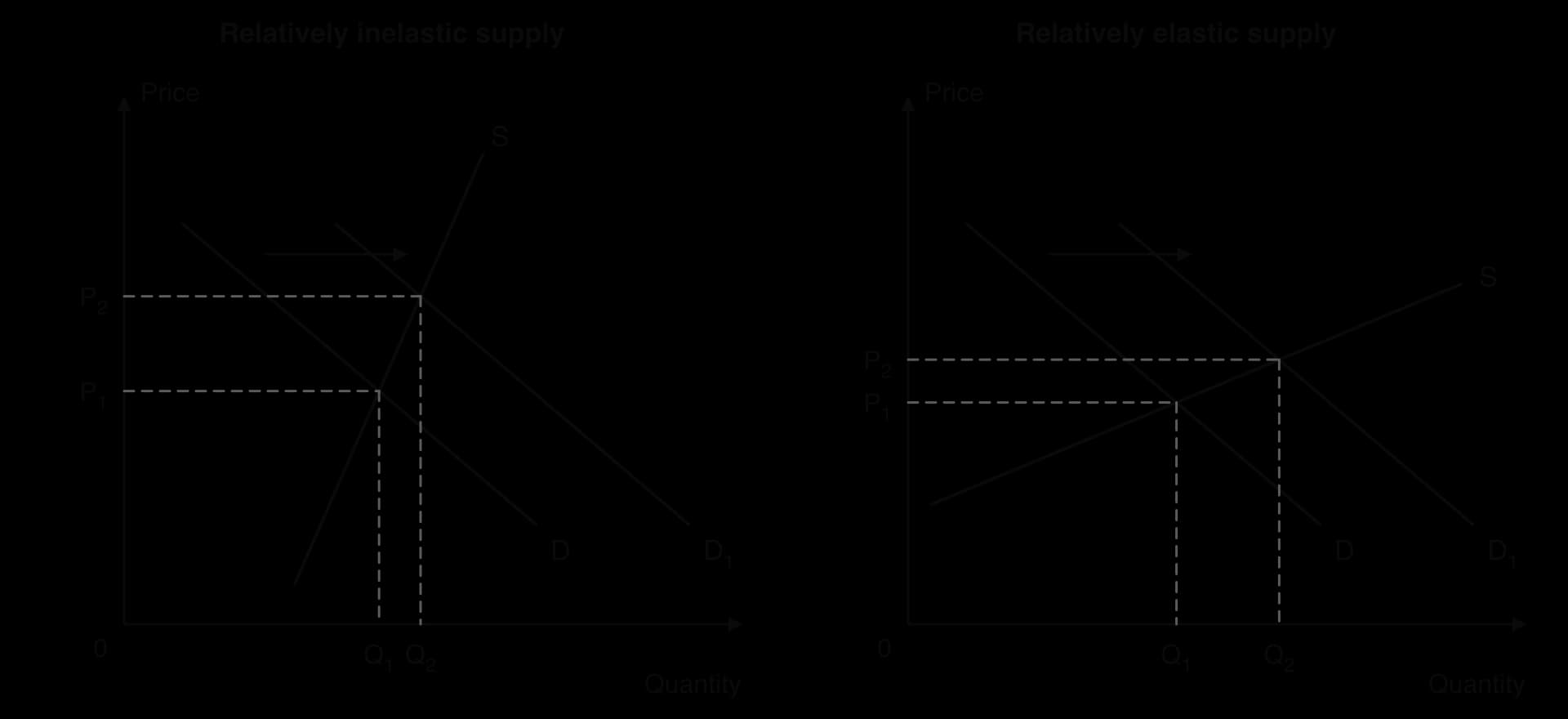
The figure shows the same rightward shift of demand in two markets. In the left panel, the steep supply curve means that producers cannot expand output much, so the new equilibrium is reached mainly through a higher price: P₁ rises a long way to P₂, while quantity rises only from Q₁ to Q₂. In the right panel, producers can expand output easily, so most of the adjustment is in quantity and the price rises only slightly.

The same logic works in reverse for a fall in demand. With inelastic supply, producers cannot cut output quickly, so the price falls sharply; with elastic supply, output is cut and the price falls only a little. Inelastic supply therefore makes prices less stable whenever demand shifts.

PES also affects government policy. The burden of an indirect tax is shared between consumers and producers depending on the relative elasticities of demand and supply: the less elastic side of the market bears more of it. When supply is very inelastic, as with land, producers bear most of a tax. Price controls are also affected: a price ceiling set below equilibrium causes a larger shortage, over time, when supply is elastic, because producers cut output more.

Governments can try to raise PES where slow supply responses cause social problems. Training programmes increase the mobility of labour; faster planning decisions and fewer restrictions on land use allow more homes to be built; strategic stocks of food or fuel allow supply to respond quickly in an emergency. Each of these raises PES but takes time and has costs of its own.

PES connects with several key concepts:

• Scarcity and choice: when supply is inelastic, a rise in demand is rationed by a higher price, and consumers must choose what to give up.

• Change: supply becomes more elastic over time, so markets adjust more fully in the long run than in the short run.

• Intervention: governments can raise PES through planning reform, training and stocks, as in Auckland’s housing reform.

• Economic well-being: inelastic supply of essentials, such as housing and energy, keeps their prices high and squeezes household budgets.

PES for primary commodities and manufactured products (HL only)

Primary commodities, such as crops, metals and energy, generally have price inelastic supply, at least in the short run. Manufactured products generally have more elastic supply. The difference follows from the determinants of PES.

Why primary commodities have low PES

• Long production times. Crops must be planted and harvested on a seasonal cycle, and tree crops take years to bear fruit: coffee arabica plants first flower three to four years after planting and take about seven years to mature fully. A new mine or oil field can take many years from discovery to production.

• Immobile factors. Land suited to coffee, cocoa or vineyards cannot be switched quickly to other uses or brought into production elsewhere, and mines and oil wells are tied to particular locations.

• Weather and nature. Farm output depends on rainfall, temperature and disease as well as on price, so producers cannot simply decide to supply more.

• Perishability and storage. Many agricultural products are perishable, and even storable commodities are costly to keep in large quantities.

• Little spare capacity. Mines and oil fields are usually run close to full capacity, so extra output requires new investment.

Manufactured goods differ on each point. Factories can usually add shifts, use spare machines and hire workers with general skills; components and finished goods can be stored; production is not tied to the weather or the growing season; and production lines can often be switched between products. Their supply is therefore more elastic, especially in the long run.

Sources: Wikipedia, “Coffea arabica” (accessed October 2026).

The 2026 oil shock shows the problem for a commodity with inelastic supply. After attacks on energy infrastructure and shipping in the Strait of Hormuz, through which about a quarter of the world’s seaborne oil trade normally passes, global oil supply fell by about 10 million barrels a day. Producers elsewhere could not replace that oil quickly, so the price adjusted instead: the Brent crude price was more than 50% higher in mid-April 2026 than at the start of the year, and it stood at about $125 a barrel in early October 2026, compared with about $70 in February.

Sources: World Bank, Commodity Markets Outlook press release (28 April 2026); FRED, Brent crude oil price DCOILBRENTEU (October 2026).

Exceptions to the general rule

The difference between commodities and manufactured goods is a tendency, not a law. Some commodities have relatively elastic supply. Storable metals and grain held in large stocks can be released quickly, and some oil producers can respond faster than others: a shale oil well in the United States can be drilled and brought into production within months, while a conventional offshore field takes years. Even so, the extra output that can be added quickly is small compared with the size of the world market, so a large supply shock still causes a large rise in price.

Some manufactured goods, in turn, have inelastic supply. Advanced microchips are made in a small number of very expensive plants that take years to build, so during the chip shortage of 2021–2022 carmakers could not obtain enough chips, and output of new cars was cut. The general rule holds because most manufacturing uses mobile factors, standard machines and storable components, while most commodity production depends on land, nature and long investment periods.

Low PED and low PES together: commodity price volatility

Demand for primary commodities is also price inelastic, because they are necessities or essential inputs with few substitutes. When both demand and supply are inelastic, any shift in either curve produces a large change in price and only a small change in quantity.

In the left panel, a poor harvest shifts supply from S to S₁. With steep demand and supply curves, the price rises from P₁ to P₂ by a large amount while the quantity falls only a little. In the right panel, the same shift in a market with elastic demand and supply raises the price only slightly; most of the adjustment is in quantity. Commodity markets are also hit by frequent supply shocks (droughts, frosts, disease, conflict) and demand shocks (booms and recessions in industrial countries), so their prices rise and fall far more than the prices of manufactured goods.

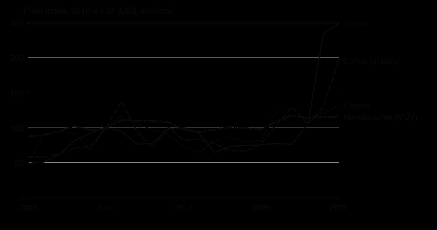
The chart compares the prices of three commodities with an index of the prices of manufactured exports (the World Bank’s MUV index), all set to 100 in 2010. Copper fell to about 65 in 2016 and rose to 132 by 2025. Arabica coffee ranged from about 58 to 196, and cocoa more than doubled between 2023 and 2025. The index for manufactured goods stayed between about 88 and 118 over the whole twenty years.

Consequences of volatile prices

Commodity price volatility creates serious problems for producers and for countries that depend on commodity exports (commodity dependence).

• Unstable incomes for producers. Farmers and miners cannot predict their income from one year to the next, which makes it hard to borrow, invest or plan, and can push poor farming households into poverty when prices fall.

• Unstable export revenue and government revenue. A country that relies on one or two commodities for most of its exports sees its export earnings, its exchange rate and its tax revenue rise and fall with world prices, making government spending and debt hard to plan.

• Weak incentives to invest. Uncertain prices discourage long-term investment in new capacity, which keeps supply inelastic.

• Overshooting. High prices encourage planting or new mines, but the extra supply arrives years later, often when prices have already fallen, deepening the next slump.

Governments and producers have tried several responses: buffer stock schemes that buy when prices are low and sell when they are high, long-term contracts and price insurance, and above all diversification of the economy into manufacturing and services. These belong to government intervention in markets and to development strategies, where they are explained and evaluated.

Case study: Auckland’s upzoning and the supply of housing

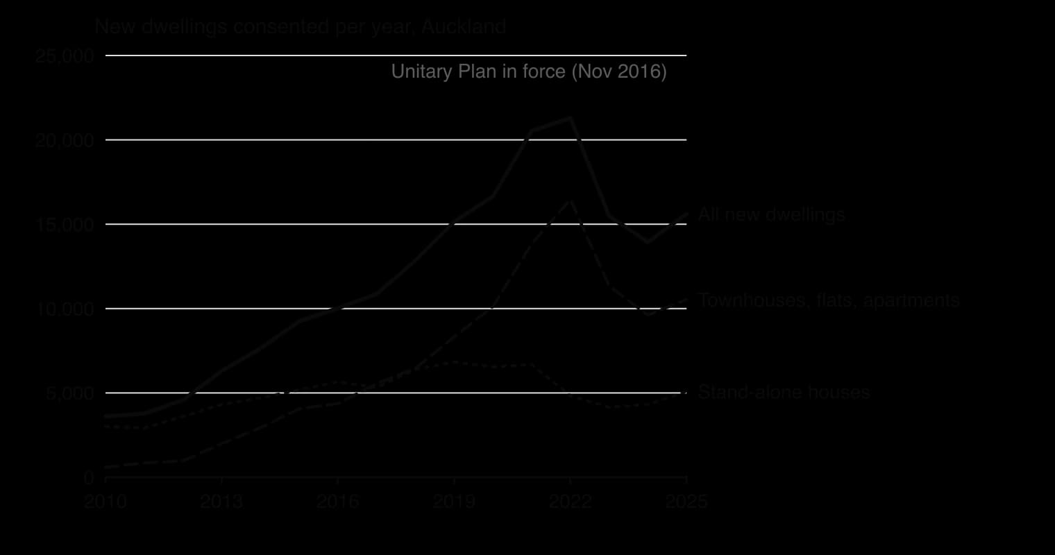
Housing supply is one of the clearest examples of inelastic supply. Building a home needs land, planning permission, materials, skilled workers and time, and in many cities rules on land use limit where and how densely homes can be built. Auckland, New Zealand’s largest city, faced rapid population growth and rising house prices in the 2010s. In November 2016 its new Unitary Plan came into force, rezoning about three-quarters of the city’s residential land to allow townhouses and apartments where previously only single, stand-alone houses had been permitted.

What happened to supply

The number of new dwellings consented in Auckland rose from 10,026 in 2016 to a record 21,301 in 2022. Almost all of the increase came from townhouses, flats and apartments, whose consents rose from 4,366 to 16,462, while consents for stand-alone houses fell. In 2022 Auckland consented 12.6 new dwellings per 1,000 residents, compared with 9.7 for New Zealand as a whole and 7.3 for the Wellington region, which had not made a similar change.

How the theory explains it

Land-use rules act on the determinants of PES. Before the reform, a developer who wanted to respond to rising prices by building more homes needed land zoned for denser housing, which was scarce and slow to obtain. In effect, land was an immobile factor and the supply curve of housing was steep. Upzoning made the existing land more mobile between uses: a plot with one old house could be redeveloped into several townhouses without a long planning process. This lowered the rate at which costs rose as output expanded and made the supply of housing more elastic.

With more elastic supply, a rise in demand for housing is met more by extra homes and less by higher prices. Economists at the University of Auckland estimated that the reform roughly doubled new dwelling consents per person within five years: over the seven years after it, about 52,200 more dwellings were consented than their estimate of what would have happened without it, 46% of the 112,300 consented. A related study estimated that rents in Auckland were about 23% lower eight years after the reform than they would otherwise have been.

Limits of the evidence

The size of the effect is disputed. The estimates compare what happened with a prediction of what would have happened without the reform, built from earlier trends and from other parts of New Zealand, and critics argue that the result depends heavily on how that prediction is made: other regions, including Wellington, also saw consents rise to a peak in 2021–2022 without a similar reform. Consents are also not completed homes; some are never built, and some replace demolished houses, so the net addition to the housing stock is smaller than the number of consents.

Consents fell back after 2022, to 15,617 in 2025, a reminder that supply also responds to the cost of borrowing and building, not only to rules on land. Even so, Auckland’s experience shows that PES is not fixed: it can be raised by policy, but only over a period of years, because building more homes takes time even when the rules allow it.

Sources: Stats NZ, Building consents issued: August 2026; Greenaway-McGrevy, _Economic Modelling (2026); Greenaway-McGrevy and So, Economic Inquiry (2026); Fresh Economic Thinking, “The Auckland myth” (accessed October 2026)._

Exam practice

PES appears in the papers in the same ways as PED. Paper 2 asks you to define PES, to calculate it from data, and to draw supply curves of different elasticity. Paper 1 asks you to explain the determinants of PES and, at HL, to explain why commodity prices are volatile. HL Paper 3 may give a straight-line supply curve and ask for the PES at a given price.

Part (b) questions often ask about policies that change PES, such as planning reform, which call for evaluation and a real example.

HL Paper 3 can test PES with a straight-line supply curve.

Summary

• PES = %ΔQs ÷ %ΔP measures how responsive quantity supplied is to a change in price; it is normally positive.

• Supply is perfectly inelastic (0), inelastic (0–1), unitary elastic (1), elastic (above 1) or perfectly elastic (∞).

• Any straight supply curve through the origin has PES = 1; one starting on the price axis is elastic, one starting on the quantity axis is inelastic.

• PES is higher the longer the time period, the more mobile the factors of production, the more spare capacity, the easier it is to store output, and the more slowly costs rise with output.

• When supply is inelastic, a rise in demand raises price a lot and quantity little; governments can raise PES through policies such as planning reform, but only over time.

• HL: primary commodities have lower PES than manufactured products (long production times, immobile land, weather, perishability), and with low PED this makes their prices volatile.

Self-check

• To do:

  I can define PES and explain why it is normally positive.

• To do:

  I can calculate PES from data and use it to find a change in price or quantity supplied.

• To do:

  I can draw relatively elastic and relatively inelastic supply curves, and perfectly elastic, perfectly inelastic and unitary elastic supply curves.

• To do:

  I can explain why every straight supply curve through the origin has a PES of 1.

• To do:

  I can explain the five determinants of PES with examples, and draw how supply becomes more elastic over time.

• To do:

  I can explain how PES affects the change in price when demand changes.

• To do:

  I can explain why PES for primary commodities is lower than for manufactured products, and why their prices are volatile (HL).