Explain the law of supply, draw supply curves for firms and markets, analyse how non-price determinants shift supply, and tell a movement along the supply curve from a shift of it.
Each is in the Economics glossary, with every other term in the subject.
The situation where producers can use the same resources to make one good or another, such as wheat or barley, so that producing more of one means producing less of the other.
The payments a firm makes for the factors of production and other inputs it uses, such as wages, rent, raw materials and energy.
The situation where producing one good automatically produces another, such as beef and leather, so that a rise in the supply of one increases the supply of the other.
The principle that, in the short run, as more units of a variable factor are added to a fixed factor, the extra output from each additional unit of the variable factor eventually falls.
The principle that, ceteris paribus, as the price of a good rises the quantity supplied rises, and as the price falls the quantity supplied falls: a positive relationship.
The period of time in which all factors of production can be varied, so firms can change their scale of production and firms can enter or leave a market.
The additional cost to a firm of producing one more unit of output.
The additional output produced when one more unit of a variable factor of production, such as one more worker, is employed.
The total quantity of a good supplied by all producers in a market at each price, found by adding the quantities that individual firms supply at that price.
A change in the quantity supplied caused only by a change in the good’s own price, shown as a move from one point to another on the same supply curve.
The factors other than the good’s own price that affect how much producers offer for sale, such as costs of factors of production, technology, taxes and subsidies, related goods, expectations and the number of firms.
The amount of a good or service that producers are willing and able to sell at one particular price during a given time period.
A change in the quantity supplied at every price, caused by a change in a non-price determinant of supply; an increase shifts the curve right and a decrease shifts it left.
The period of time in which at least one factor of production, usually capital such as buildings and machinery, is fixed in quantity.
The quantities of a good or service that producers are willing and able to offer for sale at each possible price during a given time period, ceteris paribus.
A graph showing the quantity supplied of a good at each possible price, ceteris paribus; it normally slopes upwards from left to right.
A table listing the quantity of a good supplied at each of a range of prices, for one producer or for the whole market, ceteris paribus.
The total quantity of output a firm produces with a given quantity of factors of production in a period.
Define supply and explain the law of supply, including the role of ceteris paribus.
Draw an upward-sloping supply curve from a supply schedule and label it fully.
Explain how market supply is found from the supply of individual producers.
Explain how each non-price determinant of supply (costs of factors of production, prices of related goods in joint and competitive supply, indirect taxes and subsidies, future price expectations, technology, the number of firms) shifts the supply curve.
Distinguish between a movement along the supply curve and a shift of the supply curve, using diagrams.
Explain the law of diminishing marginal returns and why it leads to increasing marginal costs (HL).
Calculate marginal product and marginal cost from data on output and wages (HL).
Supply describes how much of a good or service producers are willing and able to sell at different prices. It is the second half of every market: farmers deciding how much wheat to plant, factories deciding how many phones to assemble and hotels deciding how many rooms to open all respond to the prices they expect to receive and the costs they face.
Supply links directly to the key concepts of scarcity and efficiency. Producers use scarce factors of production (land, labour, capital and entrepreneurship), and the price they receive must cover what those resources cost. Supply theory explains how producers respond when prices, costs, technology and their circumstances change, and why some markets can respond quickly while others take years.
84 exam-style questions on this subtopic, written in the style of the IB papers. The first has its markscheme open. Counted on
Read the extract and answer the questions that follow.
Text A — New irrigation transforms rice farming in Halvenmark
[1] Halvenmark is a lower-middle-income economy in Southeast Asia. Its resources are used mainly to produce rice and simple manufactured goods such as footwear.
[2] In 2023 a government programme supplied farmers with drip-irrigation equipment and a new drought-resistant rice variety. Government scientists estimate that, if all of the country's resources were used to grow rice, the maximum harvest would now be 3.0 million tonnes a year, compared with 2.4 million tonnes before the programme. The technology has no effect on footwear production.
[3] The irrigation equipment is an example of capital. Rice harvests in 2024 and 2025 were the largest on record.
Define the term capital indicated in bold in the text (Text A, paragraph 3).
2 marks
Vague definition [1]: The idea that it is equipment or machinery.
Accurate definition [2]: An understanding that it is a man-made factor of production, such as machinery, equipment, tools or infrastructure, that is used to produce other goods and services.
N.B. Do not credit an answer that refers only to money.
Using information from Text A, paragraph 2, calculate the percentage increase in Halvenmark's maximum possible output of rice.
One of 56 short multiple-choice questions on 2.2. Pick an answer to see why it's right or wrong.
Diminishing marginal returns have set in, but marginal product is still positive. What is happening to total product?
The official deck for this part of the syllabus.
What is supply?
Which term describes: the quantities of a good or service that producers are willing and able to offer for sale at each possible price during a given time period, ceteris paribus?
With a free account, Augment remembers where you stopped and what you have practiced.
Scope: Supply belongs to the microeconomics unit at both SL and HL. SL covers the law of supply, the supply curve, individual and market supply, the non-price determinants of supply, and the difference between movements along and shifts of the curve. HL adds the theory behind the upward slope (the law of diminishing marginal returns and increasing marginal costs).
In economics, supply is not the same as the amount that exists or the amount a firm could produce. It is the amount producers are willing and able to offer for sale. A farmer with a warehouse full of grain is not supplying it if she is not prepared to sell at the current price; a factory with idle machines does not add to supply until it decides to produce.
As with demand, supply is a whole relationship between price and quantity. The amount offered at one particular price is called the quantity supplied. Keeping the two terms apart is what allows economists to tell a response to price from a change in producers’ circumstances.
The definition again relies on ceteris paribus. To isolate the effect of price, everything else that affects producers is held constant: the costs of their inputs, their technology, taxes and subsidies, the number of firms, and so on. Each of these is analysed separately as a non-price determinant.
Producers generally offer more for sale when the price is higher. When the price of wheat rises, farmers plant more of their land with wheat; when hotel room rates rise during a festival, guesthouses and homeowners offer more rooms. This positive relationship is the law of supply.
Firms are assumed to aim for profit, the difference between the revenue they earn and the costs they pay. A higher price raises the revenue from each unit, so producing more becomes more profitable. Three responses follow.
Existing firms expand output. A higher price makes it worth producing units that were too costly to produce before, for example by hiring more workers or running machines for longer.
Firms switch resources from other products. A farmer can move land from barley to wheat when wheat becomes relatively more profitable, and a clothing factory can move workers from shirts to jackets.
New firms enter the market. Over a longer period, higher prices and profits attract new producers, adding to the quantity supplied.
Behind the first response lies a fact about costs. As a firm produces more with the same factory, farm or office, the extra cost of each additional unit usually rises: workers get in each other’s way, machines are overused, and overtime must be paid at higher rates. This extra cost is the firm’s marginal cost.
Because marginal cost rises as output rises, a firm will only produce more if the price rises enough to cover the higher cost of the extra units. This is the core reason the supply curve slopes upwards. Marginal cost rises because, with some factors fixed, each extra worker eventually adds less to output than the one before.
How much producers can respond to a price change depends on how much time they have. Economists divide time into two periods, the short run and the long run, defined not by a number of months but by what can be changed.
In the short run, a bakery can hire more workers or buy more flour, but it cannot build a second oven or a bigger shop. Output can only rise by adding variable factors to the fixed ones.
The length of these periods differs between industries. A food stall might be able to change everything within weeks, while a mining company may need ten years to open a new mine. The distinction explains why supply usually responds more strongly to price in the long run than in the short run, a point measured by price elasticity of supply.
Like demand, supply can be shown as a table or a graph. The table, a supply schedule, lists the quantity supplied at several prices, for one producer or the whole market.
Price ($ per tonne) | Quantity supplied (thousand tonnes per year) |
|---|---|
150 | 20 |
200 | 40 |
250 | 60 |
300 | 80 |
The hypothetical schedule for wheat in one region shows the law of supply: each $50 rise in the price raises the quantity supplied by 20 thousand tonnes. Plotting the points gives the supply curve.
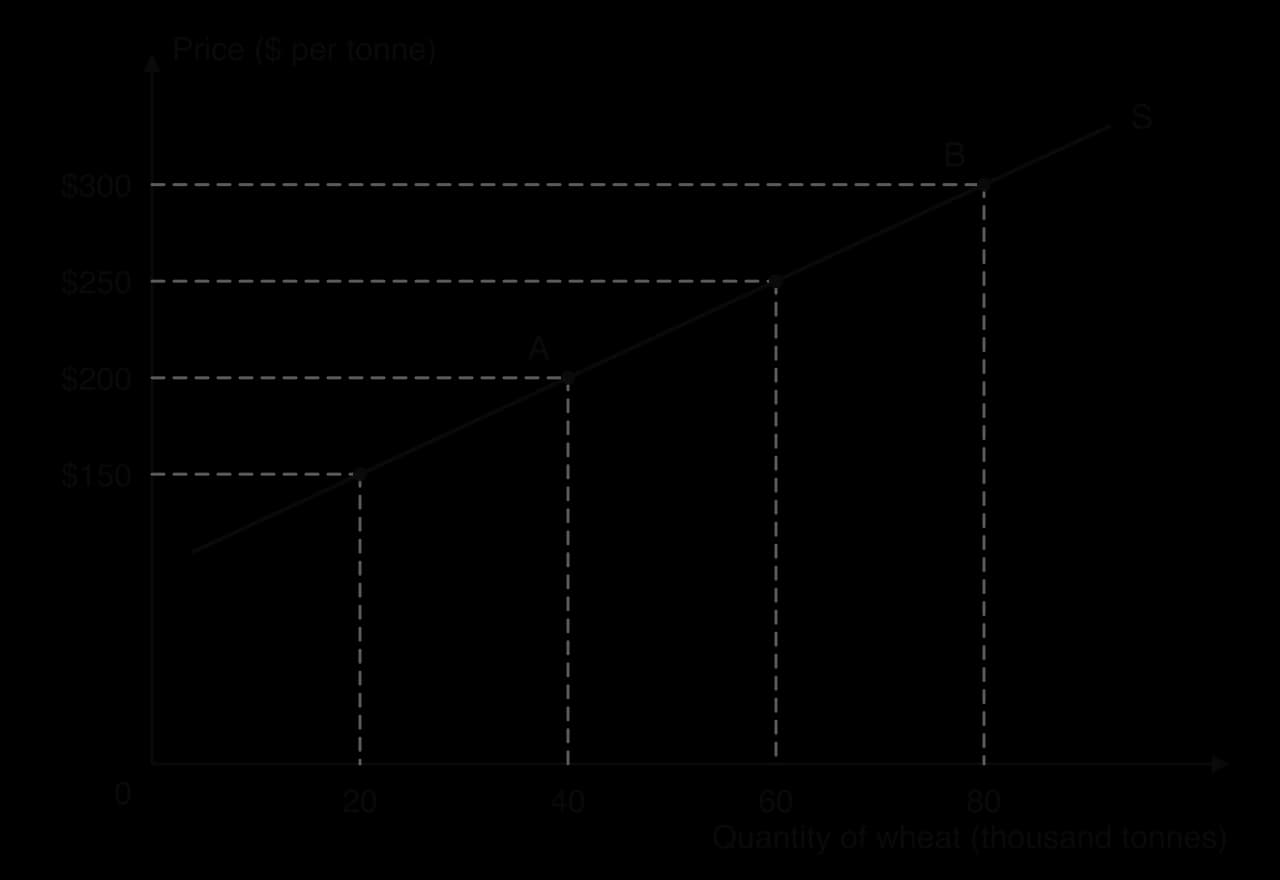
The axes follow the same convention as the demand diagram: price on the vertical axis, quantity on the horizontal axis, and the curve labelled S at its end. The move from A to B along S shows the law of supply. Supply curves, like demand curves, are usually drawn as straight lines for simplicity.
 YouTube
Each producer has its own supply curve. The supply of the whole market, market supply, is found by adding together what every producer is willing to supply at each price.
The addition is horizontal, just as for market demand. If firm A offers 12 units at $6 and firm B offers 12 units at $6, market supply at $6 is 24 units. Some firms have higher costs than others and only begin to supply once the price is high enough to cover them.
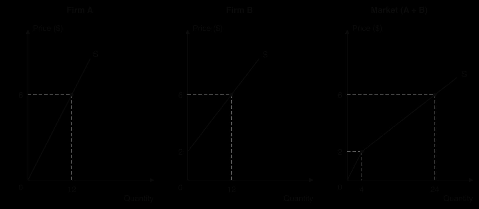
The diagram shows how the market curve combines the two firms. Below $2 only firm A, the lower-cost producer, is willing to supply. Above $2, firm B joins, and the market curve becomes flatter, because each $1 rise in price now draws extra output from two firms instead of one. With many firms, each starting at a different price, the market supply curve becomes a smooth upward-sloping line.
This link explains why the number of firms is a determinant of supply. Each new firm adds another individual supply curve to the sum, so market supply shifts to the right at every price; each firm that leaves shifts it to the left.
The law of supply rests on how costs behave as a firm produces more in the short run. When some factors of production are fixed, adding more of a variable factor eventually brings smaller and smaller increases in output, a pattern called the law of diminishing marginal returns. Each extra unit of output then costs more to produce, and firms need a higher price to cover it.
Two measures describe how output changes as a firm adds workers to fixed capital. The first is total product, the total output the firm produces. The second is marginal product, the extra output from one more worker.
A bakery with one oven provides a clear illustration (hypothetical data). The oven, the shop and the equipment are fixed in the short run; the number of bakers can change. The table shows output per day as bakers are added.
Workers | Total product (loaves per day) | Marginal product (loaves) | Marginal cost per loaf (wage $120 ÷ MP) |
|---|---|---|---|
1 | 40 | 40 | $3.00 |
2 | 100 | 60 | $2.00 |
3 | 150 | 50 | $2.40 |
4 | 190 | 40 | $3.00 |
5 | 220 | 30 | $4.00 |
6 | 240 | 20 | $6.00 |
At first, marginal product rises: a second baker allows the two to specialise, one mixing dough and one shaping and baking, so output rises by 60 loaves. From the third baker onwards, marginal product falls. There is still only one oven and limited space, so each extra worker has less capital to work with and adds less to output.
The law applies only in the short run, because it depends on at least one factor being fixed. It is a feature of production in every sector: adding fertiliser to a fixed field, waiters to a restaurant with a fixed number of tables, or programmers to a software project with a fixed deadline and system. The word “eventually” matters: marginal product may rise at first, as in the bakery, before diminishing returns set in.
If each worker costs the same wage, the cost of the extra loaves each worker produces is the wage divided by that worker’s marginal product. When marginal product is high, each extra loaf is cheap to produce; when marginal product falls, each extra loaf needs more labour time and so costs more.
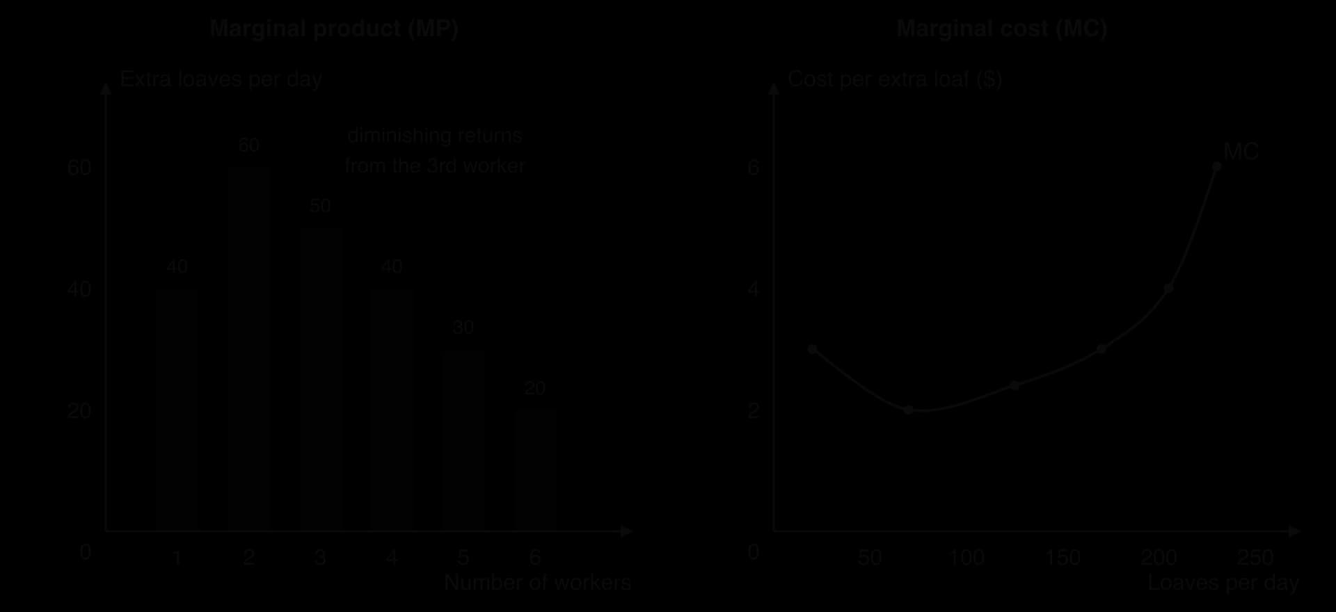
The two panels show the mirror-image relationship. While marginal product rises (workers 1 and 2), marginal cost per loaf falls from $3.00 to $2.00. Once diminishing marginal returns begin with the third worker, marginal cost rises: to $2.40, $3.00, $4.00 and finally $6.00 per extra loaf. These are increasing marginal costs.
A firm will produce an extra unit only if the price it receives is at least as high as the marginal cost of producing it. Since marginal cost rises as output rises, the firm will increase output only if the price rises. The rising part of a firm’s marginal cost curve therefore shows how much it is willing to supply at each price: it is the firm’s supply curve.
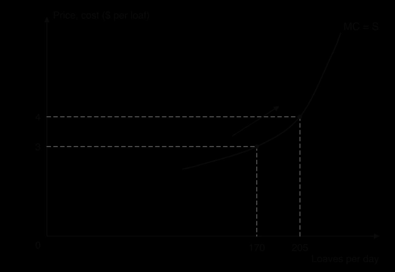
The diagram uses the bakery’s numbers, with each worker’s marginal cost plotted at the middle of the range of loaves that worker adds (the fourth baker adds loaves 151 to 190, shown at about 170).
Reading across from a price of $3 to the MC curve gives a quantity supplied of about 170 loaves, because loaves that cost more than $3 to make are not worth producing at that price. If the price rises to $4, the loaves made by the fifth baker, which cost $4 each, also become worth producing, and the quantity supplied rises to about 205 loaves. This movement up the marginal cost curve is the law of supply. Adding up the marginal cost curves of every firm gives the upward-sloping market supply curve.
 YouTube
Diminishing marginal returns explain the slope of supply in the short run. In the long run, firms can add capital as well as labour, and large firms may enjoy lower costs per unit as they grow, so long-run supply in some industries can be very flat. Some services, such as digital downloads or streaming, have marginal costs close to zero, so their supply depends more on fixed investment than on rising marginal cost. The theory fits best where output depends on fixed land or capacity, such as agriculture, mining and manufacturing in the short run.
Many factors other than price, the non-price determinants of supply, affect how much producers are willing and able to supply. When one of them changes, producers want to supply a different quantity at every price, and the whole supply curve shifts.
A shift to the right is an increase in supply: producers offer more at every price, or, equivalently, are willing to supply each quantity at a lower price. A shift to the left is a decrease in supply. A useful way to read a supply shift is vertically: if each unit costs $2 more to produce, producers need $2 more to supply each quantity, so the curve moves up by $2, which on the diagram is the same as moving to the left.
Costs of production are the payments firms make for land (rent), labour (wages), capital (interest and equipment) and raw materials and energy. A rise in any of these costs makes each unit more expensive to produce, so at each price producers supply less, and supply shifts left. A fall in costs shifts supply right.
The energy price shock of 2021–23 raised costs for energy-intensive producers such as fertiliser plants, glassworks and greenhouses in Europe, and some reduced or stopped production for a time. A rise in the minimum wage raises labour costs for restaurants and shops, which shifts their supply curves to the left. A fall in the price of cotton reduces the cost of making T-shirts and shifts their supply to the right.
Producers often make more than one product, and the price of one can affect the supply of another. The relationship works in two different ways: joint supply and competitive supply.
When the price of beef rises, farmers send more cattle to slaughter, and every animal also provides a hide. The supply of leather therefore increases at every price of leather, even though nothing has happened in the leather market itself. In the same way, refining more crude oil into petrol also produces more diesel and jet fuel.
Farmers in the United States choose each spring how to divide their land between maize (corn) and soybeans. If the expected price of soybeans rises, some farmers plant more soybeans and less maize, so the supply of maize decreases at every price of maize. A clothing factory choosing between shirts and jackets faces the same choice, with the same opportunity cost: every machine-hour used for one product cannot be used for the other.
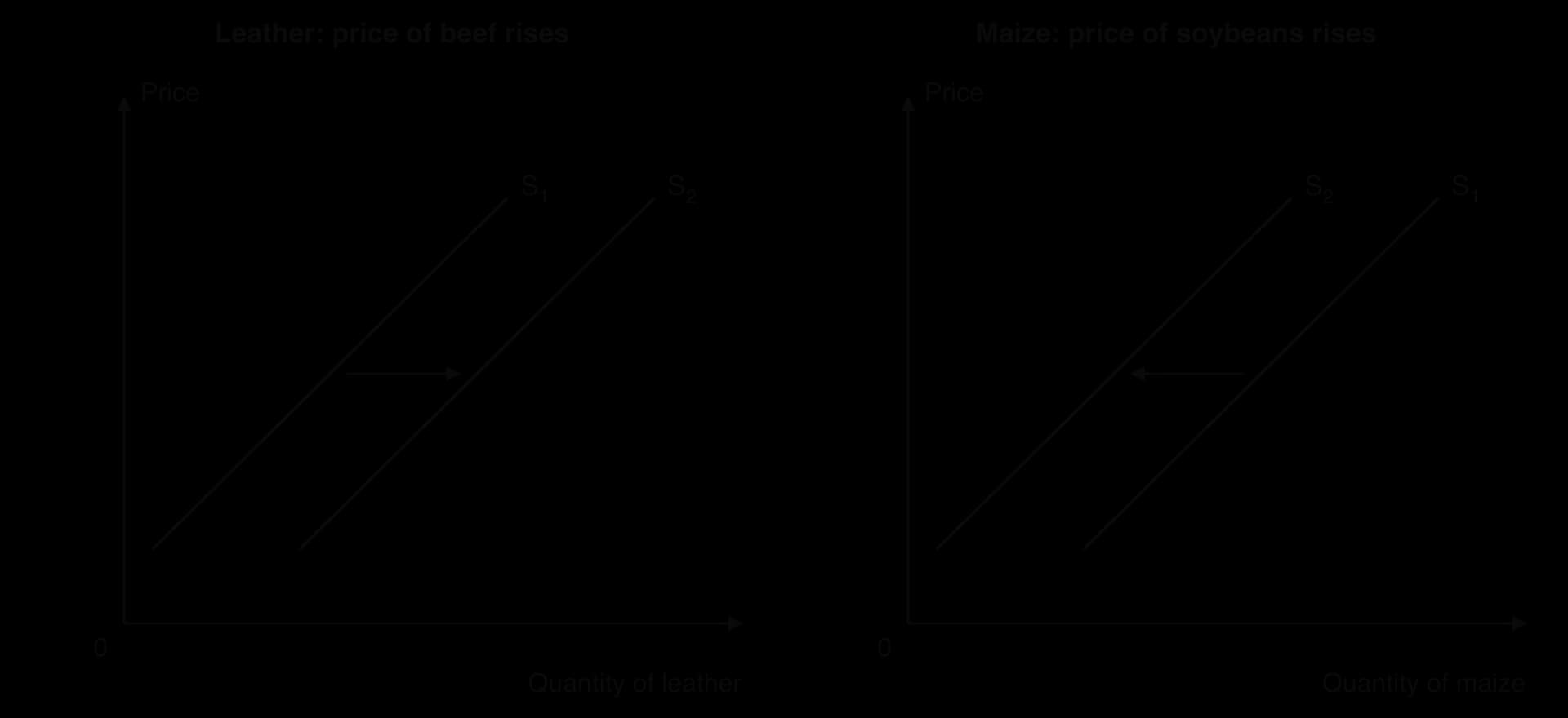
In both panels, the price of the good on the diagram has not changed, so the result is a shift of its supply curve, not a movement along it. The direction depends on the relationship: joint supply moves the two goods’ supplies together, competitive supply moves them in opposite directions.
Governments affect supply directly through taxes on goods and payments to producers. An indirect tax is a tax on spending on a good, paid to the government by the seller. To producers it works like an extra cost of production: for each unit sold, part of the price goes to the government. Supply therefore shifts to the left.
With a specific tax (a fixed amount per unit, such as $1 per packet of cigarettes), the supply curve shifts up by exactly the amount of the tax, so the new curve, S + tax, is parallel to the original. An ad valorem tax, a percentage of the price such as value added tax, shifts supply up by more at higher prices, so the new curve is steeper than the original.
A subsidy is a payment by the government to producers for each unit produced or sold. It works like a fall in costs, so supply shifts to the right: down by the amount of the subsidy per unit, to S − subsidy. Governments subsidise producers of goods they want to encourage, such as renewable energy, public transport or basic foods.
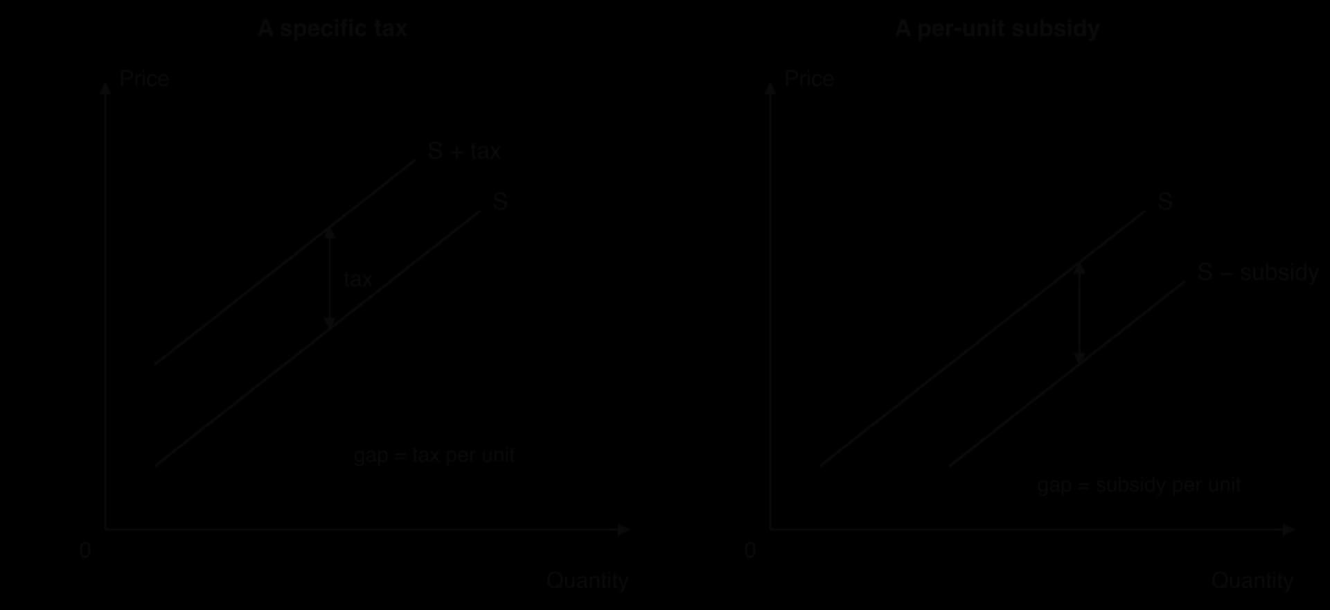
The diagram shows only the shift of supply. The full effects of taxes and subsidies on prices, quantities, consumers, producers and the government are analysed with government intervention in markets, which builds on this diagram by adding the demand curve.
Producers, like consumers, think about the future. If they expect the price of their product to rise, they may hold back some output now in order to sell it later at the higher price, which reduces supply today. If they expect prices to fall, they may try to sell as much as possible now, increasing supply today.
Farmers who can store their harvest, such as grain or coffee growers with warehouses, often delay sales when they expect prices to rise. Oil producers may also leave oil in storage when they expect higher prices later. Expectations can make supply shift even before anything has changed in current costs or technology.
Improvements in technology let producers make more output from the same inputs, or the same output with fewer inputs. This lowers costs per unit, so supply shifts to the right. Technological change is one of the main reasons that the supply of many goods, from computers to solar panels, has increased enormously over time.
Solar photovoltaic panels are a clear example. Improvements in manufacturing technology and larger, more automated factories have reduced the cost of producing solar panels dramatically since 2010, shifting supply far to the right. In agriculture, better seeds, irrigation and machinery such as the combine harvester raise the output from each hectare. Technology can occasionally reduce supply, for example when a cyber-attack or software failure stops a production line, but its usual effect is to increase it.
Because market supply is the sum of individual firms’ supply, more firms means more supply at every price. Firms enter a market when they expect to make profits there, and leave when they make losses. Entry and exit take time, so this determinant usually acts in the long run.
The growth of shale oil production in the United States after about 2010 is an example. New drilling techniques (a technology change) made it profitable to extract oil from shale rock, and thousands of new wells were drilled by a large number of producers, adding to the supply of crude oil. In the opposite direction, when many firms leave an industry, as when coal mines close, market supply shifts to the left.
Some supply shifts come from events outside producers’ control. Weather, disease and natural disasters matter most in agriculture: a drought, a frost or a plant disease reduces the harvest at every price, shifting supply left, while unusually good weather shifts it right. Wars and conflicts can disrupt supply suddenly. In 2022, Russia and Ukraine together produced about half of the world’s sunflower oil, and the Russian invasion of Ukraine in February 2022 disrupted Ukraine’s production and its exports through Black Sea ports, shifting the world supply of sunflower oil to the left. Government regulations, such as stricter safety or environmental rules, can also raise costs and reduce supply.
Sources: FAO, World Food and Agriculture – Statistical Yearbook (2025).
Non-price determinant | Change | Effect on supply of good X | Shift |
|---|---|---|---|
Costs of factors of production | Wages, raw material or energy costs rise | Decreases | Left (up) |
Price of a good in joint supply | Its price rises, so more of it is produced | Increases | Right |
Price of a good in competitive supply | Its price rises, so resources move to it | Decreases | Left |
Indirect tax | Imposed or increased | Decreases | Left (up by the tax) |
Subsidy | Granted or increased | Increases | Right (down by the subsidy) |
Future price expectations | Producers expect the price of X to rise | Decreases now | Left |
Technology | Improves | Increases | Right |
Number of firms | More firms enter the market | Increases | Right |
As with demand, every change in supply behaviour appears on a diagram in one of two ways. A change in the good’s own price causes a movement along the supply curve. A change in any non-price determinant causes a shift of the supply curve.
A shift is a different kind of change, because the quantity producers offer changes even though the price has not.
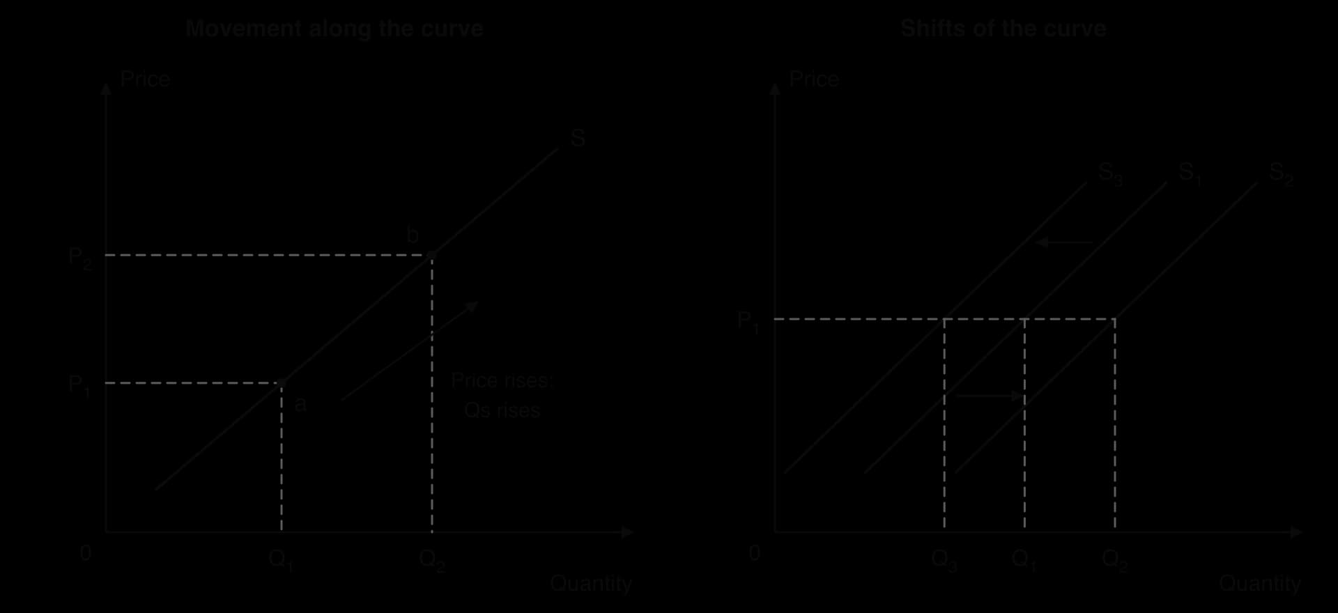
In the left-hand panel, the price rises from P₁ to P₂ and the quantity supplied rises from Q₁ to Q₂: producers respond to the higher price along their existing supply relationship. In the right-hand panel, the price stays at P₁, but producers now supply Q₂ (after an increase in supply to S₂) or Q₃ (after a decrease to S₃). Only a change in costs, technology, taxes, related prices, expectations or the number of firms can change the quantity supplied at an unchanged price.
Several key concepts are at work whenever supply changes:
Scarcity and choice: producers choose how to use scarce land, labour and capital, so competitive supply always involves an opportunity cost.
Change: technology, costs and the number of firms change constantly, shifting supply curves; time decides how fully producers can respond.
Intervention: indirect taxes and subsidies are tools governments use to reduce or increase supply.
Sustainability: climate change makes harvests less reliable, so weather-driven supply shocks such as droughts and frosts are likely to become more common.
Interdependence: a frost in Brazil or a war in Ukraine shifts supply in world markets and changes prices for consumers on other continents.
Brazil is the world’s largest coffee producer, and the state of Minas Gerais grows a large share of its arabica, the higher-quality variety. In 2021, a long drought was followed in late June and July by severe frosts across the main arabica regions. Frost damages leaves, flowers and young branches, and in severe cases kills trees outright.
Supply theory classifies this as a change in a non-price determinant: the weather. At every price, Brazilian farmers could now supply less arabica than before, so the supply curve shifted to the left. Because Brazil supplies so much of the world’s arabica, the shift affected the world market as a whole.
Marketing year (July–June) | 2017/18 | 2018/19 | 2019/20 | 2020/21 | 2021/22 | 2022/23 (forecast) |
|---|---|---|---|---|---|---|
Arabica production (million 60 kg bags) | 39.5 | 49.7 | 42.0 | 49.7 | 36.4 | 41.5 |
Total Brazilian coffee production (million 60 kg bags) | 52.1 | 66.5 | 60.5 | 69.9 | 58.1 | 64.3 |
The table shows Brazil’s arabica output, which also follows a two-year cycle: trees produce a large crop in “on-years” and a smaller one in “off-years”. The 2021/22 crop, already an off-year and hit by drought, fell to 36.4 million bags. The frosts damaged the trees that would produce the 2022/23 crop, so even though that was an on-year, arabica output was forecast at only 41.5 million bags, 8.2 million bags (about 16.5%) below the previous on-year crop of 2020/21.

The chart shows the effect on price. The monthly average price of arabica rose from 205 US cents per pound in July 2021 to 280 cents in February 2022, the highest level since 2011. The price stayed high through most of 2022 before falling back as later harvests recovered, then rose again to new records of about 410 cents in 2025.
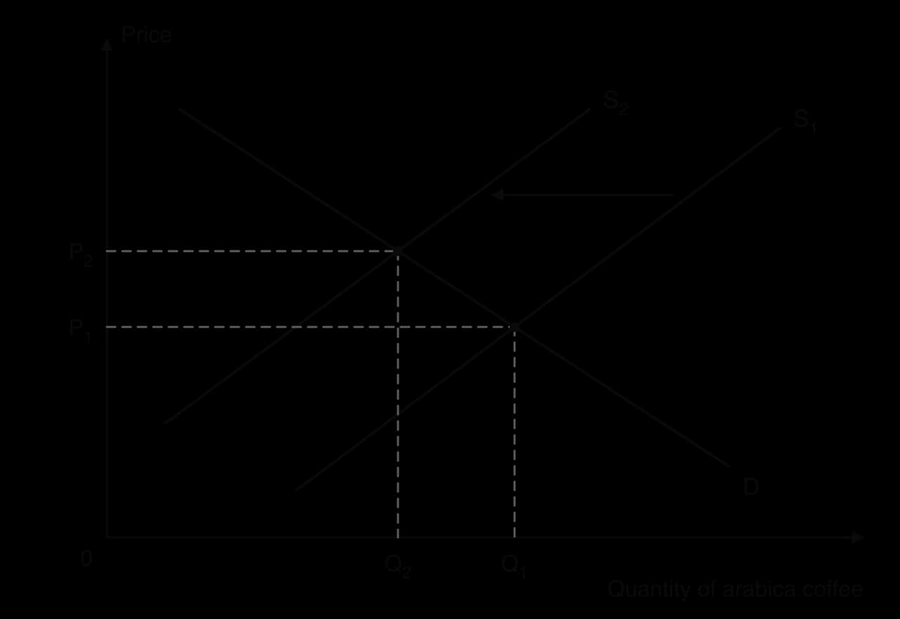
The diagram links the shift of supply to the price rise. With demand unchanged, the decrease in supply from S₁ to S₂ creates a shortage at the old price, and the price rises to P₂ at a new market equilibrium with a smaller quantity traded. This adjustment to a new equilibrium is the price mechanism at work.
Some supply shifts last a long time, and coffee shows why. It is a tree crop: severely damaged trees must be cut back or replaced, and a newly planted tree takes several years before it produces a full crop. Brazil’s stock of non-bearing (not yet productive) coffee trees rose from 1.05 billion to 1.50 billion between 2020/21 and 2021/22 as farmers replanted and pruned damaged areas. Supply could not return to its earlier position quickly, whatever the price.
The case has limits as a pure supply story. Coffee prices in 2021–22 were also affected by demand recovering after the pandemic, by shipping problems that raised freight costs, and by the exchange rate of the Brazilian real. Several determinants were changing at once, so the frost explains a large part of the price rise but not all of it. Coffee also shows the link between supply shocks and sustainability: if extreme weather becomes more frequent with climate change, shifts like this may become more common.
Sources: USDA Foreign Agricultural Service, Brazil Coffee Annual, report BR2022-0035 (June 2022); FRED, Federal Reserve Bank of St. Louis, series PCOFFOTMUSDM (2026).
Questions on supply usually test precise definitions, diagrams of shifts and movements, and short explanations of determinants. In Paper 2, definitions such as joint supply or the law of supply are worth 2 marks, and “Using an appropriate diagram, explain…” items on a shift of supply are worth 4 marks. In Paper 1, supply analysis is often the first step in explaining a change in a market’s price. HL Paper 3 can ask for calculations of marginal product and marginal cost from data, and for explanations of why diminishing marginal returns make the supply curve slope upwards.
Diagrams need to show clearly which curve moves and why, because that is where most marks for application are earned.
Short Paper 2-style items for practice:
Define the term competitive supply. [2]
Define the term market supply. [2]
Using a supply diagram, explain the effect of a fall in the price of computer chips on the supply of smartphones. [4]
Using a supply diagram, explain the effect of a per-unit subsidy on the supply of electric buses. [4]
A Paper 2 part (g)-style question for practice: “Using information from the text and your knowledge of economics, evaluate the impact of more frequent droughts and frosts on coffee producers in Brazil [15].” A strong answer uses a supply diagram, uses figures from the text (production in bags, price changes), and weighs the effects: farmers with undamaged trees gain from higher prices, while those who lost trees lose revenue for several years; consider the length of time trees take to recover, the role of irrigation and new varieties (technology), and whether production shifts to other countries.
Supply is the quantities producers are willing and able to sell at each price in a period, ceteris paribus; quantity supplied is the amount at one price.
The law of supply: price and quantity supplied are positively related, ceteris paribus, so the supply curve slopes upwards.
Market supply is the horizontal sum of individual firms’ supply at each price.
HL: in the short run, diminishing marginal returns cause increasing marginal costs, so firms need a higher price to supply more.
Non-price determinants (costs of factors of production, related goods in joint or competitive supply, indirect taxes and subsidies, future price expectations, technology, number of firms) shift the supply curve.
A change in the good’s own price causes a movement along the supply curve; a change in a non-price determinant causes a shift.
I can define supply and state the law of supply, including ceteris paribus.
I can draw and label a supply curve from a supply schedule.
I can find market supply by adding individual firms’ supply horizontally.
I can explain how each non-price determinant shifts supply, with a real example.
I can distinguish joint supply from competitive supply.
I can show how an indirect tax and a subsidy shift the supply curve.
I can show the difference between a movement along and a shift of the supply curve on a diagram.
I can explain how diminishing marginal returns lead to increasing marginal costs and an upward-sloping supply curve (HL).
I can calculate marginal product and marginal cost from data (HL).
[1] for valid working, [1] for the correct answer of 25 %.
An answer of 25 % without working is sufficient for [1].
Sketch a production possibilities curve (PPC) diagram to show the effect of the irrigation programme on Halvenmark's production possibilities (Text A, paragraph 2).
2 marks
[1] for a diagram showing the correct shift/outcome but with incorrect or missing labels; [2] for a correctly labelled diagram showing the correct shift/outcome.
The diagram should show the PPC pivoting outward on the rice axis (the rice intercept moving from 2.4 to 3.0 million tonnes), with the footwear intercept unchanged.
Axes: rice (tonnes) and footwear / manufactured goods.
A parallel outward shift of the whole PPC should be awarded [0].
Using a demand and supply diagram, explain the likely effect of the new irrigation technology on the market price of rice in Halvenmark (Text A, paragraphs 2 and 3).
4 marks
Level 1 [1–2]: There is a correct diagram OR an accurate written response.
Level 2 [3–4]: There is a correct diagram AND an accurate written response.
For Level 2, responses should include:
Diagram: a demand and supply diagram for rice with supply shifting right from S1 to S2, the equilibrium price falling from P1 to P2 and quantity rising from Q1 to Q2.
Explanation: the new equipment and seed variety raise yields per hectare and lower the cost of producing each tonne of rice, so farmers supply more at every price; with record harvests, the market price of rice falls and the quantity bought and sold rises.
Candidates who incorrectly label diagrams can be awarded a maximum of [3].
Vertical axis: price/P; horizontal axis: quantity/Q of rice.
The world market for beef is affected by changing diets and by changes in the cost of producing cattle.
Explain how one non-price determinant of demand might lower the price of beef and one non-price determinant of supply might raise it.
10 marks
Using real-world examples, discuss the consequences for stakeholders of government subsidies to livestock farmers.
15 marks
The quantity of a good that firms are willing and able to sell can change for many reasons, including changes in its own price and changes in the costs of producing it.
Explain how a rise in the price of raw materials affects the supply of a good, and why this differs from the effect of a rise in the good's own price.
10 marks
Using real-world examples, evaluate the view that an indirect tax is always paid mainly by consumers.
15 marks