A3.4 Alternative databases and data warehouses

Learning objectives

• Outline NoSQL, cloud, spatial and in-memory databases as approaches to storing data, with how each stores data, a strength, a limitation and a typical use.

• Distinguish key–value, document, wide-column and graph databases, and compare vertical with horizontal scaling and ACID with BASE.

• Explain the primary objectives of a data warehouse: subject-oriented, integrated, time-variant, non-volatile and append-only data, optimised for query performance.

• Describe how extract, transform, load (ETL) and a star schema of fact and dimension tables prepare data for analysis.

• Explain the role of online analytical processing (OLAP) in business intelligence, including the OLAP cube, roll-up, drill-down, slice and dice.

• Explain how classification, clustering, regression, association rule discovery, sequential pattern discovery and anomaly detection extract meaningful information from large data sets.

• Describe the features of distributed databases: data partitioning, replication, distribution and location transparency, global query processing, concurrency control, data consistency, fault tolerance, scalability and data security.

• Explain why data consistency is hard to maintain in a distributed database and how two-phase commit keeps ACID transactions reliable across sites.

Introduction

A single relational database on one server suits a school library or a small online shop well. Many modern systems outgrow that model: a social network stores billions of connections between people, a delivery app asks which drivers are within 2 km of a restaurant, a game updates a leaderboard thousands of times a second, and a supermarket chain wants to compare ten years of sales across hundreds of stores. Each of these needs data stored in a different shape, held in a different place, or organised for a different kind of question.

Alternative databases answer the first set of needs (NoSQL, cloud, spatial and in-memory databases). Data warehouses, online analytical processing and data mining answer the second: turning years of operational records into information that managers use to make decisions. Distributed databases spread data across many machines and sites, and must then keep every copy correct even when the network between the sites fails.

Types of database as approaches to storing data

Subtopic A3.1 described the relational database: data held in tables of rows and columns, linked by keys, queried with SQL and protected by ACID transactions. Its strengths are integrity and a single, well-defined structure. The same features become limits when data arrive in very large volumes, change shape often, or must be read by millions of users at once.

Three limits recur. First, a rigid schema means every row in a table has the same columns, so adding a new kind of attribute needs a change to the table definition, and data that varies from record to record (a product catalogue in which a shirt has sizes and a laptop has a processor speed) fits badly. Joins across many tables become slow when the tables hold billions of rows. Finally, a relational database usually runs on one main server, so handling more users means buying a bigger server, which has a ceiling. Four alternative approaches respond to these limits, each by changing one thing about a single relational database. NoSQL databases change the data model, cloud databases change where the database runs and who manages it, spatial databases add data types and indexes for location, and in-memory databases keep the working data in main memory instead of on disk.

NoSQL databases

The name NoSQL was first read as "no SQL" but is now usually expanded as "not only SQL". These systems drop the requirement that all data fit fixed tables, and many add a query language of their own that looks like SQL.

Two ideas run through every NoSQL model. The first concerns the shape of the data. Much real data is neither a tidy table nor free text, but something in between that carries its own labels.

Semi-structured data sits between the structured rows of a relational table and unstructured data such as images and free text. The second idea follows from the first. If records can carry different fields, the database cannot require one structure for all of them.

A flexible schema speeds up development, because a programmer can store a new field the moment the application needs it. It moves responsibility for consistency from the DBMS to the application: if one part of a program writes phone and another writes telephone, the database accepts both and the error appears later, when queries miss half the records.

The four NoSQL models diagram shows the same kind of customer data held in a relational table and in each of the four NoSQL models.

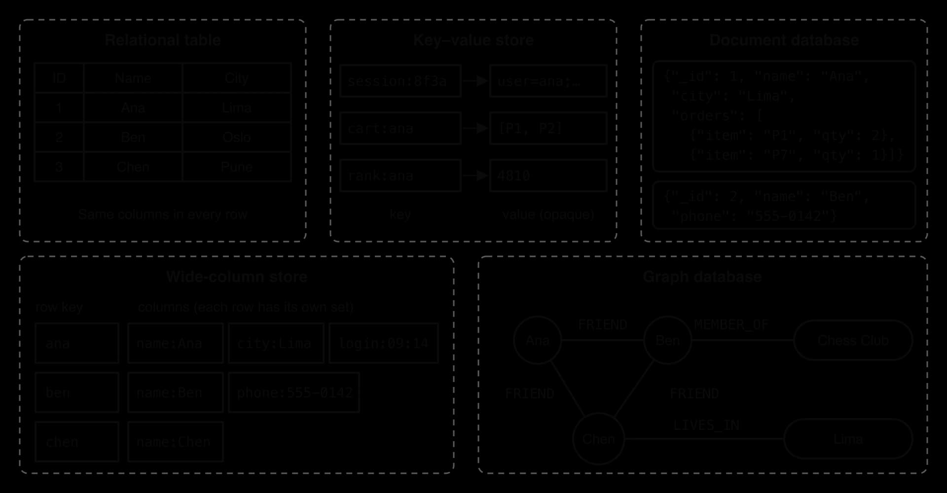
Key–value stores

A key–value store is the simplest model. Each item is a key–value pair: a unique key and a value that the database stores without interpreting. The only operations are to put a value under a key, get the value for a key, and delete a key. Because a lookup by key is a single step in a structure such as a hash table, reads and writes take about the same time however much data is stored.

The program kv.py uses a Python dictionary as a tiny key–value store holding website sessions. It shows the three operations and the model's main weakness: a question about values, such as "which sessions have an empty cart?", has no key to look up, so the program reads every item.

# A key-value store keeps each value under one unique key
store = {}

store["session:8f3a"] = "user=ana;cart=3"
store["session:91bc"] = "user=ben;cart=0"
store["session:8f3a"] = "user=ana;cart=4"   # same key: the value is replaced

print(store["session:8f3a"])
print("session:77d0" in store)

# Finding every session with an empty cart means reading every value
for key in store:
    if store[key].endswith("cart=0"):
        print("empty cart:", key)

del store["session:91bc"]
print(len(store))

import java.util.HashMap;

public class KeyValue {
    public static void main(String[] args) {
        // A key-value store keeps each value under one unique key
        HashMap<String, String> store = new HashMap<String, String>();

        store.put("session:8f3a", "user=ana;cart=3");
        store.put("session:91bc", "user=ben;cart=0");
        store.put("session:8f3a", "user=ana;cart=4");   // same key: the value is replaced

        System.out.println(store.get("session:8f3a"));
        System.out.println(store.containsKey("session:77d0"));

        // Finding every session with an empty cart means reading every value
        for (String key : store.keySet()) {
            if (store.get(key).endsWith("cart=0")) {
                System.out.println("empty cart: " + key);
            }
        }

        store.remove();
        System.out.println(store.size());
    }
}

The output is the same in both languages, except that Java prints false in lower case.

user=ana;cart=4
False
empty cart: session:91bc
1

Key–value stores suit data that is always fetched whole by one identifier: a session by session ID, a cart by user, a cached web page by URL. They suit badly any data that must be searched, filtered or joined by its contents.

Document databases

A document database stores each record as a self-contained document, usually in JSON or a binary form of it. Unlike a key–value store, the database understands the inside of each document, so it can index and query individual fields, including fields nested inside lists. A customer document can hold the customer's orders inside it, so displaying a customer page needs one read and no join.

Documents fit data with a natural "whole object" shape: product catalogues in which each product has different attributes, user profiles, blog posts with their comments, and content-management systems. The cost of embedding is duplication. If each order document copies the product's name and price, renaming a product means updating every order that mentions it, the same data redundancy problem that normalisation removes in subtopic A3.2.

Wide-column stores

A wide-column store organises data into rows identified by a row key, but each row can have its own set of columns, and a row can hold thousands or millions of them. Related columns are grouped into column families, and the data for a family is stored together on disk. Data is spread across many servers by row key, so a query that names the row key goes straight to the right server.

Wide-column stores are designed for very high write rates over huge data sets: messages in an inbox, sensor readings from millions of devices, or every event in an activity feed. A table is designed around the queries it must answer, often with the same data stored several times in different arrangements, because joins across servers are not supported.

Graph databases

A graph database stores entities as nodes and relationships as edges, both of which can carry properties ("since: 2024"). The relationship is stored as data in its own right, so following it is a direct step from one node to the next. In a relational database, the same question ("friends of my friends") needs a self-join of a large friendship table for every step, and the cost grows quickly with each extra step.

The program graph.py stores six friendships as edges and suggests new friends for Ana: people two steps away who are not already her friends. A graph database runs this kind of traversal directly over its stored edges.

# Each pair is one FRIENDS_WITH edge between two people (nodes)
edges = [["Ana", "Ben"], ["Ana", "Chen"], ["Ben", "Dev"],
         ["Chen", "Dev"], ["Chen", "Eli"], ["Dev", "Fay"]]


def friends_of(person):
    result = []
    for edge in edges:
        if edge[0] == person:
            result.append(edge[1])
        elif edge[1] == person:
            result.append(edge[0])
    return result


def suggest(person):
    direct = friends_of(person)
    suggestions = []
    for friend in direct:
        for candidate in friends_of(friend):
            if candidate != person and candidate not  direct \
                     candidate   suggestions:
                suggestions.append(candidate)
     suggestions


(, friends_of())
(, suggest())

import java.util.ArrayList;

public class Graph {
    // Each pair is one FRIENDS_WITH edge between two people (nodes)
    static String[][] edges = {{"Ana", "Ben"}, {"Ana", "Chen"}, {"Ben", "Dev"},
                               {"Chen", "Dev"}, {"Chen", "Eli"}, {"Dev", "Fay"}};

    static ArrayList<String> friendsOf(String person) {
        ArrayList<String> result = new ArrayList<String>();
        for (String[] edge : edges) {
             (edge[].equals(person)) {
                result.add(edge[]);
            }   (edge[].equals(person)) {
                result.add(edge[]);
            }
        }
         result;
    }

     ArrayList<String>  {
        ArrayList<String> direct = friendsOf(person);
        ArrayList<String> suggestions =  <String>();
         (String friend : direct) {
             (String candidate : friendsOf(friend)) {
                 (!candidate.equals(person) && !direct.contains(candidate)
                        && !suggestions.contains(candidate)) {
                    suggestions.add(candidate);
                }
            }
        }
         suggestions;
    }

        {
        System.out.println( + friendsOf());
        System.out.println( + suggest());
    }
}

Ana's friends: ['Ben', 'Chen']
Suggested for Ana: ['Dev', 'Eli']

Java prints the lists without quotation marks ([Ben, Chen]), but the contents are the same. Dev is suggested once even though he is a friend of both Ben and Chen, because the check candidate not in suggestions skips repeats. Here friends_of scans the whole edge list each time it is called; a graph database avoids that scan by storing each node's edges with the node, so a step costs the same however large the whole graph is.

YouTube

The IBM Technology video compares the four NoSQL models with a relational table, and the comparison table summarises the same points.

Scaling: vertical and horizontal

A database that receives more data and more requests must grow in capacity, its scalability. The scaling diagram shows the two ways to do this.

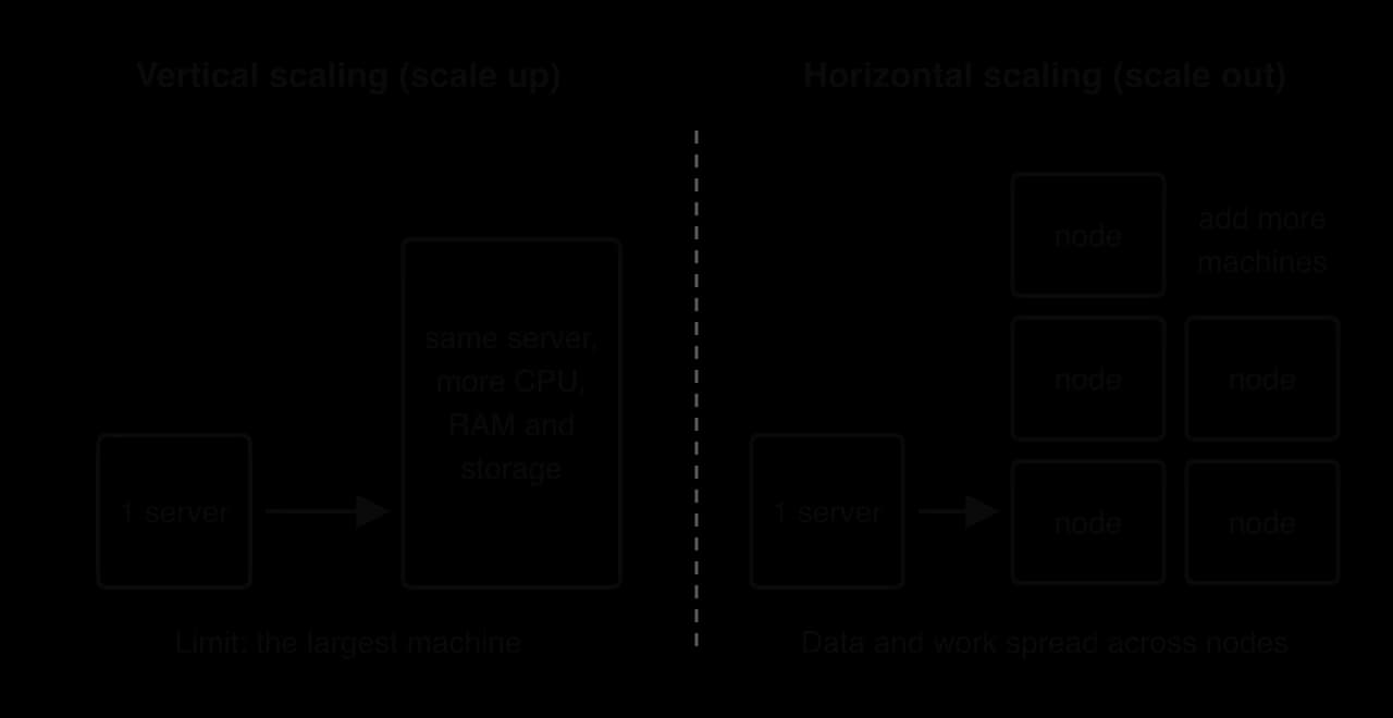
Vertical scaling needs no change to the software, keeps all data in one place and keeps transactions simple. Its limits are the price, which rises steeply for the largest machines, a hard ceiling at the biggest server available, and a single point of failure: if the one server stops, the database stops.

Horizontal scaling can continue almost without limit using ordinary, cheaper machines, and the failure of one node need not stop the system if its data is also stored elsewhere. The price is complexity: data must be divided between nodes, queries may need several nodes, and keeping copies on different nodes in step becomes hard. Most NoSQL databases were designed from the start to scale horizontally, which is a main reason large web companies adopted them; relational databases traditionally scale vertically, although distributed relational systems now exist.

Consistency models: ACID and BASE

Subtopic A3.3 showed how the ACID properties (atomicity, consistency, isolation and durability) make each transaction reliable. On one server this is affordable. When copies of the same data sit on many servers, keeping every copy identical after every write means each write must wait until all copies confirm it. If one server is slow or unreachable, writes stop. Many NoSQL systems therefore choose a weaker guarantee.

Eventual consistency is the property that sets BASE apart from ACID.

A social network can accept eventual consistency for a "like" counter: if one user sees 1,204 likes and another sees 1,203 for a second, nothing is harmed, and the site stays available even when a data centre is cut off. A bank cannot accept it for an account balance, because two cash machines reading an old balance could both pay out money that is no longer there. The choice between ACID and BASE is a choice about which failure is worse for a given application: refusing a request, or answering with data that may be out of date.

Cloud databases

A cloud database is defined by where it runs and who looks after it; its data model can be relational or NoSQL. The provider runs the database on its own servers in its data centres and offers it as a service over the internet, building on cloud computing from subtopic A1.1. The customer creates tables or collections and sends queries; the provider installs, patches, backs up, monitors and scales the system.

A managed cloud database brings several benefits. Capacity is elastic: a ticket-selling site can scale up for the minute tickets go on sale and back down afterwards. Payment is by use, so a start-up avoids buying servers. Backups, replication across data centres and security patches are automatic, so a small team does not need specialist database administrators. Many software as a service (SaaS) products, from online accounting to school management systems, store each customer's data in a cloud database for these reasons.

The limitations come from depending on someone else's infrastructure. An outage at the provider stops every application that uses it, as the DynamoDB outage of October 2025 showed. Moving to another provider can be slow and expensive (vendor lock-in). Data may be stored in another country, raising questions of data sovereignty and privacy law, and costs that look low at first can grow with heavy use. Every request also travels across the internet, adding latency compared with a database in the same building.

Spatial databases

Location is central to many systems: maps, ride-hailing apps that match riders to the nearest driver, delivery routing, emergency services, environmental monitoring and town planning. A spatial database stores geometry as a data type, so a column can hold a point (a shop), a line (a road) or a polygon (a park, a delivery zone, a country), each with coordinates.

Spatial queries ask questions that ordinary comparisons cannot answer efficiently: which restaurants are within 5 km of this customer, which delivery zone contains this address, which roads cross a flood area, which ambulance is nearest. Mapping software is the best-known application of spatial databases.

The hard part of a spatial query is speed. Checking the distance from a customer to every one of a million restaurants is a full scan. An ordinary database index sorts values along one dimension, so it cannot answer "near this point" in two dimensions. Spatial databases use a different kind of index.

An R-tree stores each object's bounding rectangle, then groups nearby rectangles into larger rectangles, level by level. A query starts at the top and descends only into the rectangles that overlap the search area, skipping whole regions at a time. The exact distance or containment test then runs only on the few objects that remain. The program spatial.py shows this two-stage idea on a small city grid: a cheap rectangle test first, then the exact distance for the survivors.

import math

# Restaurants as points on a city grid: name, x (km east), y (km north)
places = [["Noodle Bar", 2.0, 3.0], ["Taco Stop", 6.5, 1.0],
          ["Pizza Place", 9.0, 9.0], ["Green Bowl", 4.0, 7.5],
          ["Burger Shed", 7.5, 7.5], ["Curry House", 0.5, 0.5]]

home_x = 3.0
home_y = 4.0
radius = 5.0

checked = 0
for place in places:
    x = place[1]
    y = place[2]
    # Cheap test first: is the point inside the square around the circle?
    if abs(x - home_x) <= radius and abs(y - home_y) <= radius:
        checked = checked + 1
        distance = math.sqrt((x - home_x) **  + (y - home_y) ** )
         distance <= radius:
            (place[], (distance, ), )
        :
            (place[], , (distance, ), )
(, checked, , (places))

public class Spatial {
    public static void main(String[] args) {
        // Restaurants as points on a city grid: x (km east), y (km north)
        String[] names = {"Noodle Bar", "Taco Stop", "Pizza Place",
                          "Green Bowl", "Burger Shed", "Curry House"};
        double[] xs = {2.0, 6.5, 9.0, 4.0, 7.5, 0.5};
        double[] ys = {3.0, 1.0, 9.0, 7.5, , };

           ;
           ;
           ;

           ;
         (   ; i < names.length; i++) {
            
             (Math.abs(xs[i] - homeX) <= radius && Math.abs(ys[i] - homeY) <= radius) {
                checked = checked + ;
                   Math.sqrt(Math.pow(xs[i] - homeX, ) + Math.pow(ys[i] - homeY, ));
                 (distance <= radius) {
                    System.out.println(names[i] +  + String.format(, distance) + );
                }  {
                    System.out.println(names[i] + 
                            + String.format(, distance) + );
                }
            }
        }
        System.out.println( + checked +  + names.length);
    }
}

Noodle Bar 1.41 km
Taco Stop 4.61 km
Green Bowl 3.64 km
Burger Shed in the square but 5.70 km away
Curry House 4.30 km
Exact distances calculated: 5 of 6

Pizza Place fails the rectangle test, so its distance is never calculated. Burger Shed passes the rectangle test but fails the exact test, because the corners of a square lie outside the circle inside it. With six restaurants the saving is one calculation; with a million restaurants spread over a country and an R-tree to find the rectangle's contents, the database examines a few dozen candidates instead of a million. Real systems also work with latitude and longitude on a curved Earth, so the exact test uses a formula for distance on a sphere, but the two-stage strategy is the same. In a spatial database the whole search is one SQL query. The listing is a vendor-specific illustration in PostGIS syntax; it does not run in SQLite or in a standard relational database.

CREATE INDEX RestaurantLocationIdx
ON Restaurant
USING GIST (Location);

SELECT Name
FROM Restaurant
WHERE ST_DWithin(Location, ST_MakePoint(3.0, 4.0), 5.0);

ST_DWithin and ST_MakePoint are PostGIS functions and USING GIST builds an R-tree-style index; the distance 5.0 is in the units of the grid's coordinates (km here). Other spatial databases name these functions differently, and none of them is standard SQL.

In-memory databases

Main memory is far faster than secondary storage. An in-memory database keeps its whole working data set in RAM instead of on disk, so a read or write takes microseconds instead of the milliseconds a disk-based system may need when its data is not already cached.

Speed makes in-memory databases suitable for real-time work: a game leaderboard updated on every match, live stock prices, fraud checks that must finish before a card payment is approved, user sessions, and a cache that sits in front of a slower database and holds the most requested results. Real-time analytics dashboards, which recalculate figures every few seconds as new events arrive, also rely on data held in memory.

RAM is volatile: its contents disappear when the power fails. An in-memory database protects data in one of two ways, or both. It can take periodic snapshots, writing the whole data set to disk at intervals, which loses only the changes since the last snapshot. It can also append every change to a log file on disk as it happens, so the data set can be rebuilt by replaying the log after a crash, much like the transaction log in subtopic A3.3. Redis offers both methods. Other limits are cost, because RAM costs far more per gigabyte than disk, and size, because the data set must fit in the memory available, or be spread over several servers.

Data warehouses

Operational databases and analytical databases

The databases studied in subtopics A3.1 to A3.3 are operational databases. They run the business from moment to moment: recording each sale at a till, each seat booked, each grade entered. Their workload is a large number of short transactions that read or change a few rows each.

OLTP databases are normalised to 3NF so each fact is stored once and updates are safe. They usually keep only current data: when a customer changes address, the old address is overwritten. A manager who asks "how did sales of each product category change, region by region, over the last five years?" causes trouble for such a system. The history may not exist, the answer needs data from several separate systems (the tills, the online shop, the loyalty app), and the query reads millions of rows through many joins, slowing the tills for every customer while it runs.

The solution is a separate database built for analysis.

The purpose of a warehouse is decision support: giving managers and analysts reliable information about the past to plan the future.

The warehouse pipeline diagram shows where a warehouse sits in an organisation's systems.

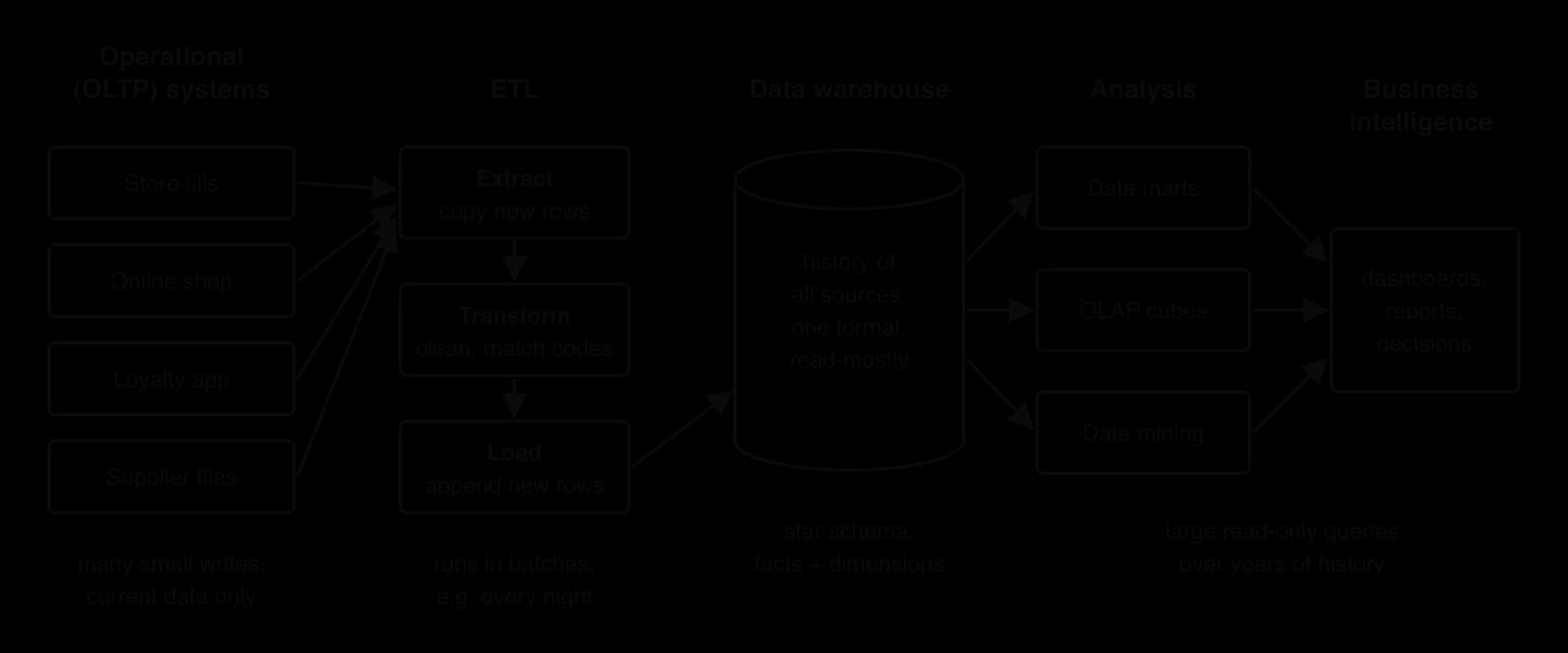
Extract, transform, load (ETL)

Data reaches the warehouse through a repeated process in three stages.

1. Extract: copy the new or changed records from each source since the last run. Sources may be relational databases, NoSQL stores, spreadsheets or files from suppliers.

2. Transform: make the data consistent. Dates take one format, currencies and units are converted, codes are matched ("M"/"F", "1"/"2" and "male"/"female" become one coding), duplicates are removed, errors are corrected or rejected, and summary values may be calculated.

3. Load: append the cleaned rows to the warehouse tables, usually in a batch at a quiet time, for example every night.

The program etl.py shows the transform stage for two sources that record the same sale differently. The tills store dates as day/month/year, products as till codes and amounts in cents; the online shop stores ISO dates, product names and amounts in euros, and one of its rows has no amount.

# Extract: rows as two source systems store them
till_rows = [["14/03/2026", "BRD-01", "240"], ["14/03/2026", "MLK-02", "115"]]
web_rows = [["2026-03-14", "bread", "2.40"], ["2026-03-15", "coffee", ""]]

product_codes = {"BRD-01": "P1", "bread": "P1", "MLK-02": "P2",
                 "milk": "P2", "CAF-03": "P3", "coffee": "P3"}

warehouse = []   # the fact rows already loaded


def till_date(text):
    # "14/03/2026" -> "2026-03-14"
    parts = text.split("/")
    return parts[] +  + parts[] +  + parts[]



clean = []
 row  till_rows:
    clean.append([till_date(row[]), product_codes[row[]], ,
                  (row[]) / ])
 row  web_rows:
     row[] == :
        (, .join(row))
    :
        clean.append([row[], product_codes[row[]], , (row[])])


 row  clean:
    warehouse.append(row)

 row  warehouse:
    (row[], row[], row[], (row[], ))

import java.util.ArrayList;
import java.util.HashMap;

public class Etl {
    static String tillDate(String text) {
        // "14/03/2026" -> "2026-03-14"
        String[] parts = text.split("/");
        return parts[2] + "-" + parts[1] + "-" + parts[];
    }

        {
        
        String[][] tillRows = {{, , }, {, , }};
        String[][] webRows = {{, , }, {, , }};

        HashMap<String, String> productCodes =  <String, String>();
        productCodes.put(, );
        productCodes.put(, );
        productCodes.put(, );
        productCodes.put(, );
        productCodes.put(, );
        productCodes.put(, );

        ArrayList<String> warehouse =  <String>();   

        
        ArrayList<String> clean =  <String>();
         (String[] row : tillRows) {
               Integer.parseInt(row[]) / ;
            clean.add(tillDate(row[]) +  + productCodes.get(row[]) + 
                    + String.format(, euros));
        }
         (String[] row : webRows) {
             (row[].equals()) {
                System.out.println( + String.join(, row));
            }  {
                   Double.parseDouble(row[]);
                clean.add(row[] +  + productCodes.get(row[]) + 
                        + String.format(, euros));
            }
        }

        
         (String row : clean) {
            warehouse.add(row);
        }

         (String row : warehouse) {
            System.out.println(row);
        }
    }
}

rejected: 2026-03-15, coffee, 
2026-03-14 P1 till 2.40
2026-03-14 P2 till 1.15
2026-03-14 P1 web 2.40

The three loaded rows now share one date format, one product code and one unit, and the incomplete web row is rejected instead of being loaded with a missing amount. Before the transform, a query for "bread sold on 14 March" would have missed one of the two sales. The division needs care in Java: Integer.parseInt(row[2]) / 100 would be integer division and turn 115 cents into 1 euro, so the listing divides by 100.0; Python's / always gives a decimal result.

The objectives of a data warehouse

Inmon's definition gives a warehouse four properties: subject-oriented, integrated, time-variant and non-volatile. Two more follow from them: data is appended rather than changed, and the structure is optimised for queries. Each property solves a specific problem of analysing operational data.

Subject-oriented data

Operational systems are organised around applications and processes: the till system, the payroll system, the online checkout. Decision-makers think in subjects: customers, products, sales, suppliers.

All sales data, whether it came from tills, the website or the phone ordering line, sits in one sales structure, so an analyst asks about sales without knowing which system recorded each one. Data needed only for running a process (a till's printer settings, a session token) is left out, keeping the warehouse focused on what decisions need.

Integrated data

Integration is the result of the transform stage of ETL. Without it, the warehouse would hold "14/03/2026" and "2026-03-14", amounts in cents and euros, and three spellings of one product, and a query would add incompatible values or miss records. With it, a report on any subject can combine data from every source and trust that like is compared with like.

Time-variant data

An operational database answers "what is true now?". A warehouse must also answer "what was true then, and how has it changed?".

Every warehouse row carries a time element: the date of a sale, the month of a stock count, the period a customer lived at an address. A warehouse typically holds five or ten years of history, compared with the current data of an OLTP system. When a customer moves house, the operational database overwrites the address; the warehouse keeps both addresses with the dates each was valid, so last year's sales are still counted in the region where they happened. Time-variant data makes trend analysis, seasonal comparisons ("this December against the last five") and forecasting possible.

Non-volatile data

Operational data changes constantly: orders are amended, stock levels go up and down. Warehouse data, once loaded, stays as it is. Because the history is never rewritten, a report run today on last year's figures gives the same answer as the same report run next month, so results can be checked, compared and audited. Read-only use also simplifies the DBMS: no locks are needed to stop users overwriting each other, so large queries run without slowing each other down.

Append-only data

Append-only storage is how a warehouse achieves non-volatility and time-variance in practice. Each ETL run adds the new period's rows; a correction is made by adding a new, dated row rather than editing the old one, so the history of what was known and when is preserved. Appending is also fast and simple, because new rows go at the end and existing indexes and summaries need only be extended. The cost is ever-growing storage, which warehouses manage by compressing or archiving very old detail while keeping summaries.

Data optimised for query performance

Analytical queries read millions of rows and summarise them with aggregate functions such as SUM and AVG. A warehouse is designed for this workload, even at the cost of storage space.

• Denormalised structure. A warehouse deliberately accepts some redundancy (denormalisation, subtopic A3.2) so that queries need fewer joins. The usual design is the star schema.

• Pre-calculated summaries. Totals by month, region and product are calculated once during loading and stored, often as materialised views, so a dashboard reads a few summary rows instead of adding up millions of sales.

• Indexes for reading. Because data is rarely written, the warehouse can carry many indexes without the cost they would add to every insert in an OLTP system.

• Column-oriented storage. Many warehouse systems store each column's values together on disk, so a query that sums one column out of fifty reads only that column.

Star schemas: fact tables and dimension tables

The structure most warehouses use separates the measurements of a business process from the descriptions of its context.

A fact table is long and narrow: it can hold billions of rows, each mostly numbers and keys. The descriptions of who, what, where and when are kept in separate tables.

The fact table joined to its dimension tables forms the shape that gives the design its name. The star schema diagram shows a supermarket's sales warehouse.

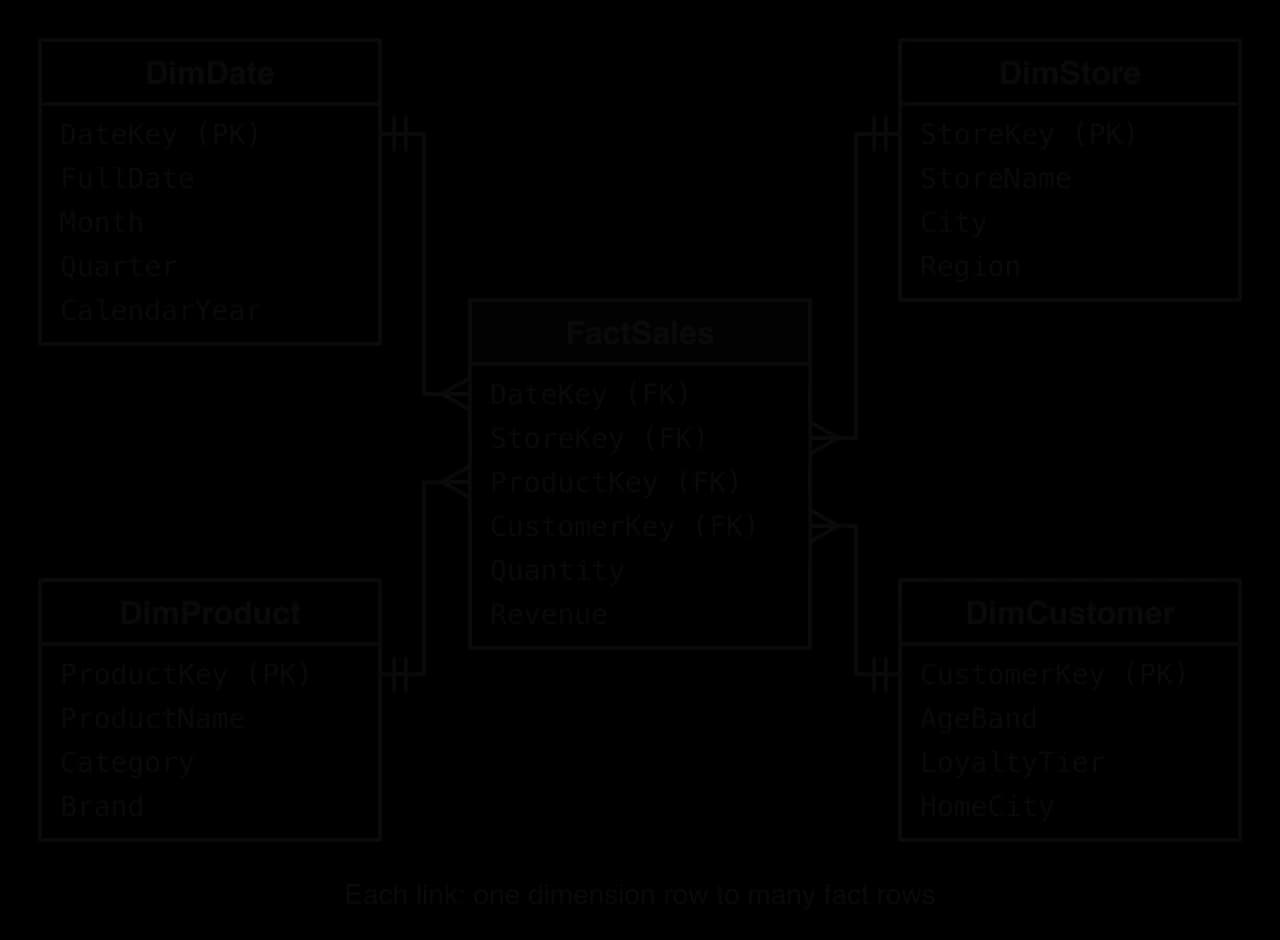
DimStore holds City and Region in every store's row, although a normalised design would put regions in a separate table. That redundancy is acceptable because the warehouse is non-volatile: the anomalies that normalisation prevents arise when data is updated, and warehouse data is not updated. DimDate breaks each date into month, quarter and year so that grouping by any of them needs no date calculation. The query groups revenue by quarter and region using one join to each dimension it needs.

SELECT d.Quarter, s.Region, SUM(f.Revenue) AS TotalRevenue
FROM FactSales AS f
INNER JOIN DimDate AS d ON f.DateKey = d.DateKey
INNER JOIN DimStore AS s ON f.StoreKey = s.StoreKey
GROUP BY d.Quarter, s.Region
ORDER BY d.Quarter, s.Region;

A small sample of eight sales, shown with the dimension values each fact row's keys point to, is enough to test it.

The query groups these eight rows into one row per quarter and region and adds up the revenue in each group.

A warehouse covering the whole organisation can be large and slow to change, so departments often work from a smaller extract.

A marketing data mart might hold only customer and campaign data, giving that team faster queries and simpler tables. Marts built separately from the main warehouse risk becoming inconsistent with each other, which is why many organisations load marts from the central warehouse so that every department starts from the same integrated data.

OLAP and data mining for business intelligence

A warehouse full of clean history is only useful if people can extract information from it. Two families of tools do this: OLAP, in which a person asks questions and explores the answers interactively, and data mining, in which algorithms search the data for patterns no one asked about.

OLTP and OLAP

YouTube

The IBM Technology video contrasts the two kinds of processing, which differ on almost every point.

The OLAP cube

OLAP tools present warehouse data as a cube. Each axis is a dimension (product, region, quarter) and each cell holds measures (sales, quantity) for one combination of dimension values. A real cube usually has more than three dimensions (a hypercube), but the three-dimensional picture shows the idea.

Analysts explore a cube with a small set of operations. Moving between levels of detail is the most common.

Choosing part of the cube is the other main operation.

The OLAP cube diagram applies each operation to a small supermarket cube.

A further operation, pivot, rotates the cube so that a different pair of dimensions forms the rows and columns of the display, like rearranging a spreadsheet pivot table. In SQL terms, a slice or dice is a WHERE condition on dimension attributes, and a roll-up is a GROUP BY on fewer or coarser attributes. Drilling down from the quarter-and-region result to individual stores for Q1 in the North adds StoreName to the grouping:

SELECT s.StoreName, SUM(f.Revenue) AS TotalRevenue
FROM FactSales AS f
INNER JOIN DimDate AS d ON f.DateKey = d.DateKey
INNER JOIN DimStore AS s ON f.StoreKey = s.StoreKey
WHERE d.Quarter = 'Q1' AND s.Region = 'North'
GROUP BY s.StoreName
ORDER BY s.StoreName;

The result splits the 492.50 for Q1 North into its two stores: Hilltop 400.50 and Riverside 92.00. The program olap.py carries out a roll-up and a slice on the twelve cells of the cube diagram.

# Each fact: quarter, region, product, sales in thousands of euros
facts = [["Q1", "North", "Bread", 40], ["Q1", "North", "Milk", 25],
         ["Q1", "North", "Coffee", 30], ["Q1", "South", "Bread", 35],
         ["Q1", "South", "Milk", 30], ["Q1", "South", "Coffee", 20],
         ["Q2", "North", "Bread", 45], ["Q2", "North", "Milk", 20],
         ["Q2", "North", , ], [, , , ],
         [, , , ], [, , , ]]


by_region = {}
 fact  facts:
    region = fact[]
     region   by_region:
        by_region[region] = 
    by_region[region] = by_region[region] + fact[]
(, by_region)


q2_by_product = {}
 fact  facts:
     fact[] == :
        product = fact[]
         product   q2_by_product:
            q2_by_product[product] = 
        q2_by_product[product] = q2_by_product[product] + fact[]
(, q2_by_product)

import java.util.HashMap;

public class Olap {
    public static void main(String[] args) {
        // Each fact: quarter, region, product; sales (thousands of euros) in a parallel array
        String[][] facts = {{"Q1", "North", "Bread"}, {"Q1", "North", "Milk"},
                            {"Q1", "North", }, {, , },
                            {, , }, {, , },
                            {, , }, {, , },
                            {, , }, {, , },
                            {, , }, {, , }};
        [] sales = {, , , , , , , , , , , };

        
        HashMap<String, Integer> byRegion =  <String, Integer>();
         (   ; i < facts.length; i++) {
               facts[i][];
             (!byRegion.containsKey(region)) {
                byRegion.put(region, );
            }
            byRegion.put(region, byRegion.get(region) + sales[i]);
        }
        System.out.println( + byRegion);

        
        HashMap<String, Integer> q2ByProduct =  <String, Integer>();
         (   ; i < facts.length; i++) {
             (facts[i][].equals()) {
                   facts[i][];
                 (!q2ByProduct.containsKey(product)) {
                    q2ByProduct.put(product, );
                }
                q2ByProduct.put(product, q2ByProduct.get(product) + sales[i]);
            }
        }
        System.out.println( + q2ByProduct);
    }
}

Roll-up to region: {'North': 195, 'South': 175}
Slice Q2, by product: {'Bread': 75, 'Milk': 55, 'Coffee': 60}

Java's HashMap does not keep the order in which keys were added, so the Java version prints the same totals in a different order. Because adding up is the only operation, the program uses an accumulator per group, exactly the work that SUM with GROUP BY does in SQL.

Data mining

With OLAP, analysts answer questions they have already thought of. Large data sets also contain patterns no one has thought of: groups of customers who behave alike, products that sell together, early signs that a machine will fail. Finding them by hand is impossible when the data runs to billions of rows.

Data mining uses pattern recognition at a scale no person can manage. Six techniques cover most business uses. The first four are also kinds of machine learning task, taught in subtopic A4.1, and the algorithms behind them are explained in subtopic A4.3; for business intelligence what matters is what each one finds and why the finding is useful.

Classification

Classification assigns each record to one of a set of known categories, using a model learned from past records whose category is already known (labelled data). A bank trains a classifier on past loans labelled "repaid" or "defaulted" and uses it to classify new applications; a phone company classifies customers as "likely to leave" or "likely to stay" (churn) and offers the first group a discount. Its value to the business is a prediction about each individual case before the outcome is known.

Clustering

Clustering divides records into groups whose members are similar to each other and different from other groups, without any labels: the groups are discovered, not given. A retailer clusters customers by what, when and how often they buy, and might find a "weekday lunchtime" group and a "weekend family" group, each of which receives different offers. The value is in discovering segments the business did not know existed.

Regression

Regression predicts a continuous numeric value from other values: next month's sales from advertising spending and season, a house price from its size and location, how many staff a store needs on Saturday. Classification predicts a category and regression predicts a number. In business intelligence, regression supports forecasting, budgeting and stock planning.

Association rule discovery

Association rule discovery finds items or events that occur together in the same transaction, and expresses each pattern as an association rule "if X, then Y". Its best-known use is market basket analysis of supermarket receipts. Two measures judge a rule. Support is the fraction of all transactions that contain every item in the rule; it shows how common the pattern is. Confidence is the fraction of transactions containing X that also contain Y; it shows how reliable the rule is.

A supermarket uses strong rules to place products, design bundle offers and suggest items online ("customers who bought this also bought…").

Sequential pattern discovery

Association rules ignore order: a rule built from receipts says that two items appear in the same basket, not which came first. Many business questions are about order over time: what customers buy after a first purchase, which pages lead to a sign-up, which machine readings come before a breakdown.

The data for sequential pattern discovery is a set of sequences, one per customer (or user, or machine), each a time-ordered list of events. A sequential pattern such as ⟨phone, then case within 30 days⟩ is counted for a customer if that customer's sequence contains the first event and later the second, within the window. The support of the pattern is the fraction of customers whose sequence contains it. Patterns with high support become business actions: email a case offer to every new phone buyer during the first month, or recommend the next course a student usually takes.

The program seq.py counts the customers who bought a phone and then a case within 30 days.

# Purchase history: customer, day number, item
events = [["C1", 3, "phone"], ["C1", 10, "case"],
          ["C2", 5, "case"], ["C2", 20, "phone"],
          ["C3", 1, "phone"], ["C3", 45, "case"],
          ["C4", 12, "phone"], ["C4", 13, "charger"], ["C4", 30, "case"],
          ["C5", 7, "laptop"]]
customers = ["C1", "C2", "C3", "C4", "C5"]
first_item = "phone"
then_item = "case"
window =    

matches = 
 customer  customers:
    found = 
     a  events:
         a[] == customer  a[] == first_item:
             b  events:
                gap = b[] - a[]
                 b[] == customer  b[] == then_item   < gap <= window:
                    found = 
     found:
        matches = matches + 
        (customer, )

support = matches / (customers)
(, support)

public class Seq {
    public static void main(String[] args) {
        // Purchase history: customer, day number, item (three parallel arrays)
        String[] who = {"C1", "C1", "C2", "C2", "C3", "C3", "C4", "C4", "C4", "C5"};
        int[] day = {3, 10, 5, 20, , , , , , };
        String[] item = {, , , , , ,
                         , , , };
        String[] customers = {, , , , };
           ;
           ;
           ;   

           ;
         (String customer : customers) {
               ;
             (   ; a < who.length; a++) {
                 (who[a].equals(customer) && item[a].equals(firstItem)) {
                     (   ; b < who.length; b++) {
                           day[b] - day[a];
                         (who[b].equals(customer) && item[b].equals(thenItem)
                                && gap >  && gap <= window) {
                            found = ;
                        }
                    }
                }
            }
             (found) {
                matches = matches + ;
                System.out.println(customer + );
            }
        }

           () matches / customers.length;
        System.out.println( + support);
    }
}

C1 follows the pattern
C4 follows the pattern
Support of <phone, then case within 30 days>: 0.4

The trace of each customer shows why only two of five match.

C2 bought both items, so an association rule built on whole purchase histories would count C2; the sequential pattern does not, because the order is wrong. In Java, (double) matches / customers.length converts before dividing, otherwise integer division would give 0.

Anomaly detection

Most records in a large data set follow normal patterns; a few do not. Those few are often the most important: a stolen card used abroad, a network intrusion, a faulty sensor, a data-entry error that adds three zeros to a price.

The simplest approach is statistical. Calculate the mean and standard deviation of a measure, then calculate each value's z-score, its distance from the mean in standard deviations; values whose z-score is beyond a chosen threshold are flagged as outliers.

More advanced systems learn what is normal for each customer or device separately, combine many features (amount, place, time of day, merchant type, how quickly payments follow each other) and use clustering (a record far from every cluster is suspicious) or classification models trained on past confirmed fraud. The program anomaly.py applies the z-score method to one customer's card payments.

import math

# One customer's card payments in euros, oldest first
amounts = [24.50, 31.00, 18.75, 42.00, 27.30, 35.10, 22.80, 29.95, 950.00, 33.40]
threshold = 2.5   # flag anything more than 2.5 standard deviations from the mean

total = 0.0
for amount in amounts:
    total = total + amount
mean = total / len(amounts)

squares = 0.0
for amount in amounts:
    squares = squares + (amount - mean) ** 2
std_dev = math.sqrt(squares / len(amounts))

print("mean", format(mean, ".2f"), "standard deviation", format(std_dev, ".2f"))
for amount in amounts:
    z = (amount - mean) / std_dev
    if abs(z) > threshold:
        print("ANOMALY:", format(amount, ), , (z, ))

public class Anomaly {
    public static void main(String[] args) {
        // One customer's card payments in euros, oldest first
        double[] amounts = {24.50, 31.00, 18.75, 42.00, 27.30, 35.10, 22.80, 29.95, 950.00, 33.40};
        double threshold = 2.5;   // flag anything more than 2.5 standard deviations from the mean

        double total = 0.0;
        for (double amount : amounts) {
            total = total + amount;
        }
           total / amounts.length;

           ;
         ( amount : amounts) {
            squares = squares + Math.pow(amount - mean, );
        }
           Math.sqrt(squares / amounts.length);

        System.out.println( + String.format(, mean)
                +  + String.format(, stdDev));
         ( amount : amounts) {
               (amount - mean) / stdDev;
             (Math.abs(z) > threshold) {
                System.out.println( + String.format(, amount)
                        +  + String.format(, z));
            }
        }
    }
}

mean 121.48 standard deviation 276.24
ANOMALY: 950.00 z = 3.00

The 950-euro payment is flagged. The output also shows the method's main weakness. The anomaly itself pulls the mean up from about 29 to 121 and inflates the standard deviation, which lowers its own z-score. With only ten values no z-score can exceed 3 (the maximum is $\sqrt{n - 1}$ for $n$ values), so a threshold of 3 would never flag anything here. Practical systems therefore use measures less affected by extreme values, such as the median and interquartile range, or compare each payment with the customer's long-term history.

Every anomaly detector trades two kinds of error. A low threshold catches more fraud but blocks more honest payments (false positives), which annoys customers; a high threshold lets more fraud through (false negatives). The bank chooses the threshold by weighing the cost of each error, and a flagged payment usually triggers a check (a text message to the customer) rather than an automatic accusation.

Comparing the techniques

OLAP, data mining and their limits

OLAP and data mining complement each other. OLAP is user-driven and verifies what an analyst already suspects ("did the new store layout raise sales in the South?"); data mining is data-driven and discovers patterns to test next. A typical workflow uses mining to find a pattern, such as a customer cluster with falling spending, and OLAP to explore it by region, product and month before deciding what to do.

Both depend entirely on the data underneath. Errors that ETL fails to remove lead to wrong totals and false patterns. Mining also finds correlations, not causes: a rule linking two products does not show that placing them together will raise sales, which a controlled trial would need to confirm. With very large data sets, some patterns appear by chance alone, so discovered patterns are checked on new data before anyone acts on them.

Mining personal data raises ethical questions, developed in subtopic A4.4. Customer profiles can reveal sensitive facts that customers never disclosed, such as health conditions inferred from purchases. Models trained on past decisions can repeat past unfairness, for example a credit classifier that learns to disadvantage applicants from certain postcodes (algorithmic bias). Data protection laws in many countries require a lawful purpose for processing, limits on how long data is kept, and the right of people to see the data held about them.

Distributed databases

What a distributed database is

The databases of subtopics A3.1 to A3.3 sit, logically, in one place. A global company cannot work that way: customers in Tokyo should not wait for every query to cross the Pacific to a server in Virginia, a single server cannot hold or process data for hundreds of millions of users, and one building is a single point of failure for a fire, a power cut or a cut cable.

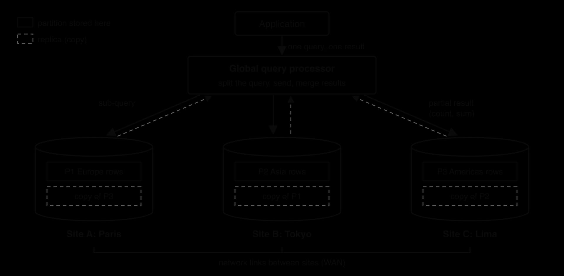
A distributed database is a kind of distributed system, subtopic A2.1. Each site runs its own DBMS software, and a layer of distributed database software coordinates them so that applications send ordinary queries and receive ordinary results. The distributed database diagram shows three sites holding a company's order data.

Data partitioning

Partitioning determines which data is stored at which site.

Horizontal partitioning splits a table by rows according to a partitioning key. In range or list partitioning the key's value determines the site directly: orders from Europe go to Paris, orders from Asia to Tokyo. In hash partitioning a hash function of the key determines the site, for example CustomerID MOD 3, which usually spreads rows evenly across the sites. Vertical partitioning splits a table by columns: a customer's name and address might sit at one site, and their large, rarely read photo or their sensitive payment details at another, each copy keeping the primary key so rows can be rejoined.

Good partitioning puts data near the users who need it most, so most queries run at one site, and spreads the load so no site is overloaded. Poor partitioning creates a "hot spot": if customers are partitioned by surname initial, the site holding names beginning with S is far busier than the one holding X, Y and Z. Queries that need data from several partitions are slower, because they cross the network.

Replication

Partitioning alone would make each partition depend on one site: if Tokyo fails, every Asian order is unavailable. Replication adds copies.

Replication improves availability and fault tolerance, because any surviving replica can serve the data, and read performance, because reads are spread across replicas and served near the user. It costs storage and network traffic, and every write must reach every replica, which raises the problem of keeping them identical.

• Synchronous replication confirms a write only when all replicas have stored it. Every read then sees the latest value, but each write waits for the slowest replica, and a write cannot complete if a replica is unreachable.

• Asynchronous replication confirms a write once one copy has stored it and sends it to the other replicas afterwards. Writes are fast and continue during network problems, but a read from a lagging replica can return old data, the eventual consistency of BASE, and if the first copy fails before sending the update on, that update can be lost.

Transparency

A distributed database is only practical if programmers and users can treat it like one database. Hiding the distribution is called transparency.

Distribution transparency has several parts: users need not know how tables are partitioned (fragmentation transparency), that copies exist (replication transparency), or where each part is stored. The last is the most commonly named.

With location transparency, a programmer writes SELECT * FROM Orders WHERE OrderID = 88123 and the system finds the site holding that order. Without it, the program would need to name the Tokyo server, and moving a partition to a new site would break every program that refers to it. Transparency is a form of abstraction: the details of placement are hidden behind a simple interface, so they can change without affecting the applications.

Global query processing

When a query needs data from several sites, the system plans how to answer it.

The global query processor (often running on the site that received the query) uses a catalogue of where each partition and replica is stored. It selects the sites to ask, sends each a sub-query, and merges what comes back. Because the network is usually the slowest part, a good plan does as much work as possible at each site and sends back only small results: for a total, each site returns its own sum instead of every row. The distributed database diagram shows this flow for an average order value, and the program gq.py simulates it.

# Orders are partitioned horizontally: each site holds its own region's rows
regions = ["Europe", "Asia", "Americas"]
site_rows = [[40.0, 55.0, 35.0, 50.0],
             [80.0, 120.0],
             [30.0, 25.0, 45.0, 60.0, 40.0, 20.0]]


def local_part(rows):
    # Runs at each site: returns only a count and a sum, not every row
    total = 0.0
    for amount in rows:
        total = total + amount
    return [len(rows), total]


# Coordinator: send the sub-query to every site, then merge the partial results
count = 0
total = 0.0
for i in range(len(regions)):
    part = local_part(site_rows[i])
    print(regions[i], "site returns count", part[0], , part[])
    count = count + part[]
    total = total + part[]

(, total / count)

public class GlobalQuery {
    // Runs at each site: returns only a count and a sum, not every row
    static double[] localPart(double[] rows) {
        double total = 0.0;
        for (double amount : rows) {
            total = total + amount;
        }
        double[] result = {rows.length, total};
        return result;
    }

    public static void main(String[] args) {
        // Orders are partitioned horizontally: each site holds its own region's rows
        String[] regions = {"Europe", "Asia", "Americas"};
        double[][] siteRows = {{, , , },
                               {, },
                               {, , , , , }};

        
           ;
           ;
         (   ; i < regions.length; i++) {
            [] part = localPart(siteRows[i]);
            System.out.println(regions[i] +  + () part[]
                    +  + part[]);
            count = count + () part[];
            total = total + part[];
        }

        System.out.println( + total / count);
    }
}

Europe site returns count 4 and sum 180.0
Asia site returns count 2 and sum 200.0
Americas site returns count 6 and sum 220.0
Global average order value: 50.0

Each site returns two numbers instead of its rows. The sites return a count and a sum, not their own averages, because an average of averages is wrong when the partitions differ in size: the three site averages are 45, 100 and about 36.67, whose mean is about 60.56, but the true average of all twelve orders is $600 / 12 = 50$. AVG is not decomposable, while COUNT and SUM are, so a global query processor rewrites AVG into a SUM and a COUNT at each site.

Data consistency and concurrency control across sites

Data consistency means every user sees data that obeys the database's rules and every copy agrees. On one server, concurrency control with locks ensures that two transactions do not overwrite each other. Across sites the same goal is harder for three reasons:

• Replicas: an update must reach every copy, or users at different sites read different values.

• Transactions spanning sites: moving money from an account in Paris to one in Lima changes data at two sites, and both changes must happen or neither.

• Partial failure: one site, or the network link to it, can fail while the others continue, so a site can be part-way through a transaction when it loses contact.

Distributed concurrency control extends the methods of subtopic A3.1. With distributed locking, a transaction obtains locks at every site it touches, often through a lock manager, before changing data; the risk is a deadlock spread across sites that no single site can see. Timestamp ordering gives each transaction a globally agreed timestamp and applies conflicting operations in timestamp order, which needs clocks at different sites to agree closely. Google's Spanner, described in 2012, uses GPS receivers and atomic clocks in its data centres for this purpose, so that transactions on different continents can be ordered consistently.

ACID across sites: two-phase commit

ACID was designed for one database. In a distributed transaction, atomicity is the hardest property: each site can commit or roll back its own part, but the transaction as a whole must not commit at Paris and roll back at Lima. The standard solution is a protocol in which a coordinator asks every site to promise before anyone commits.

The two-phase commit diagram shows the messages for a transaction that commits.

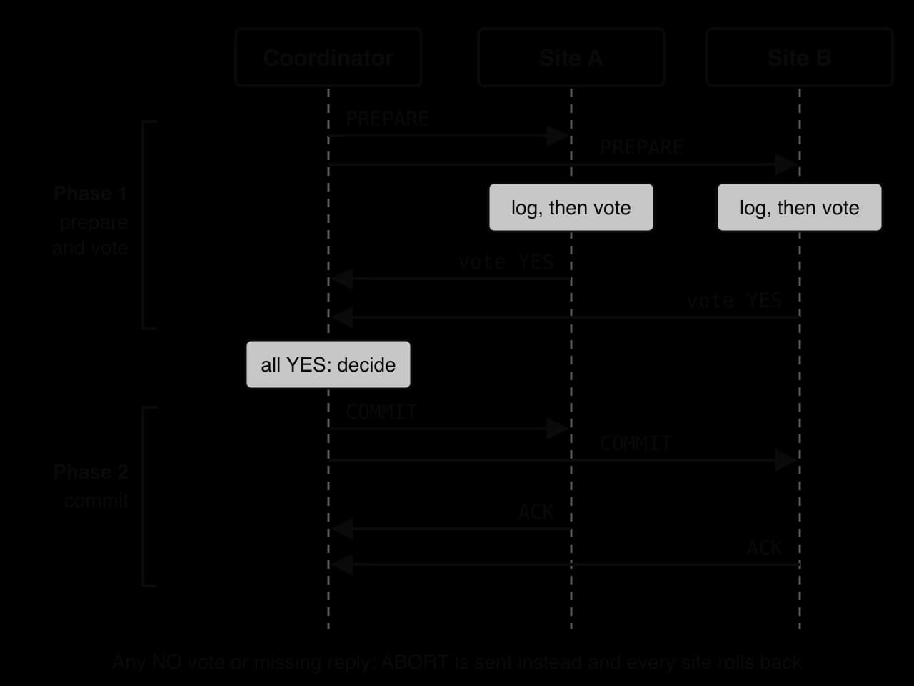
1. Phase 1 (prepare and vote). The coordinator sends PREPARE to every participating site. Each site carries out its part of the transaction, writes the changes to its transaction log so they survive a crash, holds its locks, and votes YES (it can commit) or NO (it cannot, for example because a constraint failed).

2. Decision. If every vote is YES, the coordinator records COMMIT in its own log; if any vote is NO, or a site does not reply in time, it records ABORT.

3. Phase 2 (commit or abort). The coordinator sends the decision to every site. Each site commits or rolls back its part, releases its locks and acknowledges.

The program tpc.py simulates the coordinator's decision for two transfers between three sites.

def two_phase_commit(sites, votes):
    # Phase 1 (prepare): every site does its part, writes it to its log, and votes
    decision = "COMMIT"
    for i in range(len(sites)):
        print("  PREPARE sent to", sites[i], "- vote:", votes[i])
        if votes[i] != "YES":
            decision = "ABORT"
    # Phase 2 (commit or abort): the one decision goes to every site
    for site in sites:
        print("  ", decision, "sent to", site)
    return decision


sites = ["Paris", "Tokyo", "Lima"]
print("Transfer 1:", two_phase_commit(sites, ["YES", "YES", "YES"]))
print("Transfer 2:", two_phase_commit(sites, ["YES", "NO", "YES"]))

public class TwoPhaseCommit {
    static String twoPhaseCommit(String[] sites, String[] votes) {
        // Phase 1 (prepare): every site does its part, writes it to its log, and votes
        String decision = "COMMIT";
        for (int i = 0; i < sites.length; i++) {
            System.out.println("  PREPARE sent to " + sites[i] + " - vote: " + votes[i]);
            if (!votes[i].equals("YES")) {
                decision = "ABORT";
            }
        }
        // Phase 2 (commit or abort): the one decision goes to every site
        for (String site : sites) {
            System.out.println("   " + decision + " sent to " + site);
        }
        return decision;
    }

        {
        String[] sites = {, , };
        String[] allYes = {, , };
        String[] oneNo = {, , };
        System.out.println( + twoPhaseCommit(sites, allYes));
        System.out.println( + twoPhaseCommit(sites, oneNo));
    }
}

  PREPARE sent to Paris - vote: YES
  PREPARE sent to Tokyo - vote: YES
  PREPARE sent to Lima - vote: YES
   COMMIT sent to Paris
   COMMIT sent to Tokyo
   COMMIT sent to Lima
Transfer 1: COMMIT
  PREPARE sent to Paris - vote: YES
  PREPARE sent to Tokyo - vote: NO
  PREPARE sent to Lima - vote: YES
   ABORT sent to Paris
   ABORT sent to Tokyo
   ABORT sent to Lima
Transfer 2: ABORT

In Transfer 2, Paris and Lima were ready to commit, but one NO from Tokyo makes every site roll back. Two-phase commit is how each ACID property survives distribution. Atomicity: all sites commit or none does. Consistency: a site votes NO if its part would break a rule. Isolation: every site keeps its locks until the decision arrives. Durability: sites write to their logs before voting, so a site that crashes after voting YES can recover and complete the commit.

The protocol has costs. Every distributed transaction needs at least two rounds of messages across the network, so it is slower than a local commit. Worse, it can block: a site that has voted YES must keep its locks and wait until it hears the decision. If the coordinator crashes after collecting the votes but before sending the decision, those sites cannot safely commit or roll back on their own, and the locked data stays unavailable until the coordinator recovers. This is one reason many large-scale systems avoid distributed transactions where they can.

The CAP theorem (extension)

With two-phase commit, transactions stop when a site cannot be reached, so consistency is kept at the cost of availability. Some systems are designed to keep answering instead. The CAP theorem, an extension to the core material on distributed databases, states the trade-off precisely.

Network partitions happen in any real wide-area system, so the real choice is what to do during one. A CP system refuses or delays requests that it cannot answer with the latest data: suitable for bank balances, stock levels and seat bookings. An AP system answers every request with the data it has and reconciles copies when the network recovers, accepting eventual consistency: suitable for social media feeds, product reviews and shopping-cart contents. When there is no partition, a system can provide both consistency and availability. The "C" in CAP means that all replicas agree; it is not the same as the "C" in ACID, which means that a transaction obeys the database's rules.

Fault tolerance, scalability and data security

The remaining features come from combining partitioning and replication.

• Fault tolerance. Replicas at several sites mean the failure of a node, or a whole data centre, does not lose data or stop the service: requests move to a surviving replica (failover). Logs let a failed site recover and catch up. Fault tolerance has limits: replicas that all depend on one shared service fail together.

• Scalability. More capacity is added by adding nodes (horizontal scaling) and moving some partitions to them. Read capacity grows with more replicas; write capacity grows with more partitions.

• Data security. Data travels between sites over networks, so it is protected by encryption in transit and at rest. Access control must be applied consistently at every site, because an attacker needs only the weakest site. Placing data in several countries raises data sovereignty questions: personal data about citizens of one country may be required by law to stay within it, which partitioning by region can satisfy.

• Performance and the network. Local queries are fast; queries and transactions that span sites depend on the latency and bandwidth of the links between them, and every replica or commit protocol adds network traffic.

The features table summarises how each feature is achieved and what it costs.

Case study: the Amazon DynamoDB outage of October 2025

Amazon DynamoDB is a managed NoSQL key–value database, announced in 2012, that Amazon Web Services (AWS) runs for its customers; it claims single-digit-millisecond latency for simple reads and writes by key. It is a cloud database in the full sense: customers never see a server, and AWS handles partitioning, replication across availability zones (separate data centres within a region) and scaling. Many of AWS's own services also store their data in it.

On 19 October 2025 at 11:48 PM Pacific time, applications in AWS's US-EAST-1 region (Northern Virginia) suddenly could not connect to DynamoDB. The cause was a latent race condition in the automation that manages DynamoDB's DNS records, the records that turn DynamoDB's regional endpoint name into the IP addresses of its load balancers. The component that applies DNS plans runs as three independent copies, one in each of three availability zones, for resilience. Two of them interfered: a delayed copy applied an old plan over a newer one, and the other copy's clean-up process then deleted that old plan as out of date. The regional endpoint was left with an empty DNS record, and the automation could not repair it without manual intervention by engineers.

Source: Amazon Web Services, "Summary of the Amazon DynamoDB Service Disruption in the Northern Virginia (US-EAST-1) Region", October 2025.

The stored data was never damaged and remained replicated as designed; the failure was in the DNS records that direct requests to it. For about 2 hours 52 minutes no one could reach DynamoDB in the region, and the disruption to services built on top of it lasted about 14 hours 32 minutes in total. Customers of DynamoDB's global tables, which replicate a table to other regions, could keep working against their replicas elsewhere, although replication to and from Virginia lagged. Services that depended on DynamoDB failed in turn, including EC2 instance launches and Amazon Redshift, AWS's own data warehouse service, whose query processing relies on DynamoDB endpoints. Websites and apps around the world that run on AWS were affected.

The incident illustrates several ideas about cloud and distributed databases:

• Fault tolerance has a scope. Each protection guards against one kind of failure, and an error in infrastructure shared by every replica (here the regional DNS name) bypasses all of them.

• Cloud databases concentrate dependence. A managed service removes the work of running a database, but thousands of organisations then share one provider's failure, and a fault in one region spreads to services elsewhere that depend on it.

• Concurrency is hard even for the provider. The root cause was a race condition between two copies of a component designed to improve resilience, the same kind of problem concurrency control in databases is designed to prevent.

• Design choices for customers. Organisations that replicated critical data to a second region, or across providers, recovered faster, at the cost of more complexity and expense.

AWS's response was to disable the DNS automation worldwide until the race condition was fixed and extra protections were added, and to add controls limiting how much load-balancer capacity automatic health checks can remove at once.

Exam focus

Alternative databases and data warehouses are HL only and are examined in Paper 1 Section A, as extra question parts added to an SL database question or as HL parts set in a scenario such as a retailer, bank, streaming service or ride-hailing company. The content statements use outline (database types: a brief account of what each is and how it is used, one or two sentences per mark), explain (data warehouse objectives, OLAP and data mining: a feature plus the reason or consequence) and describe (features of distributed databases: a detailed account of how each works). Short parts of 2–4 marks ask you to outline a NoSQL model or a database type for a given use, distinguish OLTP from OLAP, or explain one warehouse property; longer parts of 4–6 marks ask how a company could use a data mining technique, or describe how a distributed database stays consistent and fault-tolerant. Calculations can appear: support and confidence, roll-ups of a cube, or a global average from partitioned data.

Questions about distributed databases often name a feature and ask you to describe it. Use the exact term and its mechanism, and keep the related terms apart: partitioning divides data, replication copies it, transparency hides its placement, and two-phase commit keeps a transaction atomic across sites.

Calculation parts (support and confidence, cube roll-ups, global averages) give marks for the method as well as the answer, so write the fraction or sum before the result and state the unit or percentage.

Practice questions

1. State what the letters in BASE stand for. [1]

2. Outline one reason a social media platform might store its users' connections in a graph database rather than a relational database. [2]

3. Distinguish between vertical scaling and horizontal scaling. [2]

4. Explain why a cloud database is not a NoSQL data model, and outline one risk of using one. [3]

5. Explain why a data warehouse is integrated, with reference to ETL. [3]

6. Describe the structure of a star schema. [3]

7. A cube holds sales by product, store and month. Identify the OLAP operation that (a) shows only March; (b) moves from monthly to yearly totals; (c) shows two products in three stores over four months. [3]

8. In 1,000 shopping baskets, 200 contain pasta and 150 contain both pasta and sauce. Calculate the support and confidence of {pasta} ⇒ {sauce}. [2]

9. Distinguish between location transparency and distribution transparency. [2]

10. Explain how two-phase commit ensures atomicity in a distributed database, and describe one disadvantage of the protocol. [5]

Summary

• NoSQL databases use non-relational models with flexible schemas: key–value stores (fetch by key), document databases (JSON-like documents), wide-column stores (rows with their own columns) and graph databases (nodes and edges). Most scale horizontally and many use BASE with eventual consistency instead of strict ACID.

• Vertical scaling enlarges one server; horizontal scaling adds servers and spreads data and work across them.

• A cloud database is a hosting model (often a managed service) with elastic capacity and no hardware to run, but dependence on the provider, the network and data location rules. Spatial databases store geometry and use spatial indexes (R-trees) for location queries; in-memory databases keep data in RAM for speed and use snapshots or logs against its volatility.

• A data warehouse holds subject-oriented, integrated, time-variant, non-volatile, append-only data loaded by ETL and optimised for queries, usually as a star schema of a fact table and dimension tables.

• OLTP runs many short transactions on current data; OLAP analyses historical data interactively through an OLAP cube with roll-up, drill-down, slice and dice.

• Data mining discovers patterns automatically: classification (known categories), clustering (natural groups), regression (numbers), association rules (items together, with support and confidence), sequential patterns (events in order over time) and anomaly detection (records that do not fit).

• A distributed database stores data at several sites but appears as one: partitioning divides data, replication copies it, distribution and location transparency hide its placement, and global query processing splits queries and merges partial results.

• Keeping data consistent across sites needs distributed concurrency control and two-phase commit, which makes transactions atomic across sites at the cost of extra messages and possible blocking; the CAP theorem (an extension) states that during a network partition a system must choose between consistency and availability.

Self-check

• To do:

  I can outline NoSQL, cloud, spatial and in-memory databases, each with how it stores data, a strength, a limitation and a real use.

• To do:

  I can match a scenario to a key–value, document, wide-column or graph database and justify the choice.

• To do:

  I can explain why "NoSQL" does not mean "no SQL" and why a cloud database is not a data model.

• To do:

  I can compare vertical and horizontal scaling, and ACID with BASE and eventual consistency.

• To do:

  I can explain how a spatial index avoids checking every object in a location query.

• To do:

  I can explain each of the six objectives of a data warehouse with its benefit, and say what "non-volatile" means here.

• To do:

  I can describe the three stages of ETL and give examples of transformations.

• To do:

  I can construct a star schema for a scenario, with a fact table, measures and dimension tables.

• To do:

  I can distinguish OLTP from OLAP and apply roll-up, drill-down, slice and dice to a cube, including calculating totals.

• To do:

  I can explain what each of the six data mining techniques finds and how a business could use it.

• To do:

  I can calculate support and confidence, the support of a sequential pattern and a z-score.

• To do:

  I can describe data partitioning, replication, distribution and location transparency, and global query processing.