Calculate and interpret the mean, median, mode, quartiles, interquartile range and standard deviation, present data in bar charts, pie charts and infographics, and spot misleading charts in business data.
Each is in the Business glossary, with every other term in the subject.
A chart in which data for separate categories are shown as bars of equal width whose lengths are proportional to the values, drawn horizontally or vertically.
Numerical measures and charts that summarise and present the main features of a set of data, such as its typical value (average) and its spread.
A visual presentation that combines charts, icons, short text and key figures to communicate information quickly to a general audience.
A measure of spread equal to the upper quartile minus the lower quartile, showing the range of the middle 50% of a set of ordered data.
A chart that plots values against time, or another continuous variable, as points joined by lines, used to show trends and changes over time.
The sum of all the values in a data set divided by the number of values; the arithmetic average.
The middle value of a data set when the values are arranged in order of size; with an even number of values, the mean of the two middle values.
The value or category that occurs most often in a set of data.
Define descriptive statistics and explain why businesses use them.
Calculate the mean, median and mode of a data set and explain when each is the most useful average.
Calculate the range, quartiles and interquartile range of a data set.
Explain the meaning of standard deviation and calculate it for a small data set.
Construct and interpret bar charts and pie charts, and explain the use of infographics.
Explain how charts can mislead and choose an appropriate chart for a set of data.
Apply descriptive statistics to decisions in human resources, finance, marketing and operations.
Businesses collect large amounts of numerical data: sales by product and region, survey responses, wages, delivery times, defect rates. Descriptive statistics summarise such data in a few numbers and charts, so that managers can see what is typical, how much the data vary and how one group compares with another.
Statistics shape decisions about people and money, which links them to ethics. A pay report that quotes the mean rather than the median, or a chart with a stretched axis, can give a misleading picture to employees, customers or investors even when every number in it is correct.
60 exam-style questions on this subtopic, written in the style of the IB papers. The first has its markscheme open. Counted on
Brightwell Schools is a private company that runs two international schools in Malaysia. The principal of the Kuala Lumpur campus, Mr Tan, makes all major decisions himself and expects teachers to follow school policies closely. The principal of the Penang campus, Dr Nair, sets up teacher working groups to decide on timetables, assessment and school events. In June 2026 all teachers completed the same staff survey. Each statement was scored from 1 (strongly disagree) to 10 (strongly agree).
Table 1: Mean scores for each survey statement, by campus
Survey statement | Kuala Lumpur | Penang |
|---|---|---|
I enjoy working at this school | 5.2 | 7.4 |
I feel trusted to do my job well | 4.8 | 7.9 |
I understand what is expected of me | 6.1 | 6.8 |
My views are considered before decisions are made | 3.9 | 8.1 |
I would recommend this school as an employer | 5.5 | 7.3 |
Using Table 1, calculate the mean score across the five statements for each campus (show all your working).
2 marks
The official deck for this part of the syllabus.
Define the term descriptive statistics.
State the three things descriptive statistics reduce a large data set to.
With a free account, Augment remembers where you stopped and what you have practiced.
A value in a data set that is much higher or much lower than most of the other values, either a genuine unusual case or an error in the data.
The value below which a given percentage of the values in an ordered data set lie; the 50th percentile is the median and the 25th and 75th are the quartiles.
A circular chart divided into sectors, each showing one category’s share of a whole, with the angle of each sector proportional to that share.
One of the three values that divide a set of ordered data into four equal parts: the lower quartile (Q1), the median (Q2) and the upper quartile (Q3).
A measure of spread equal to the difference between the highest and the lowest values in a data set.
A distribution of data that is not symmetrical, with a longer tail on one side; in a positively skewed distribution the tail is to the right and the mean is greater than the median.
A measure of the spread of a data set that shows how far, on average, the values lie from the mean; a larger standard deviation means more widely spread data.
A list of 500 survey responses or 12 months of daily sales is hard to read. Descriptive statistics reduce it to a few figures: an average that represents a typical value, a measure of how spread out the values are, and a chart that shows the pattern at a glance. They describe the data that have been collected; they do not by themselves prove why the data look as they do.
Data can be numerical (quantitative), such as prices, ages and weekly sales, or categorical (qualitative), such as customers’ favourite brand, region or method of payment. Most averages and measures of spread apply only to numerical data, while the mode and most charts can be used for both types. The data may describe a whole population (every employee of a firm) or a sample drawn from it (200 customers out of 50,000), in which case the statistics are estimates for the population.
An average is a single value that represents the centre of a set of data. Three averages are in common use, and each answers a slightly different question: the mean shows the value each item would have if the total were shared equally; the median is the middle value; the mode is the most common value.
The mean uses every value, so it reflects the whole data set and can be used in further calculations: a manager who knows the mean order value and the number of orders can work out total sales revenue. Because it uses every value, however, it is pulled towards extreme values. One very large order can raise the mean order value well above what a typical customer spends.
To find the median, the values are first put in order. With values, the median is the value in position . With 9 values it is the 5th; with 10 values the position is 5.5, so the median is halfway between the 5th and 6th values. The median ignores how large the highest and lowest values are, so it is not distorted by extreme values.
The mode is the only average that can be used for categorical data, such as the most popular colour or the most common reason customers give for a complaint. A data set can have one mode, two modes (bimodal) or none, if every value occurs equally often. For a retailer deciding what to stock, the mode is often the most useful average: it shows which size, flavour or model sells most.
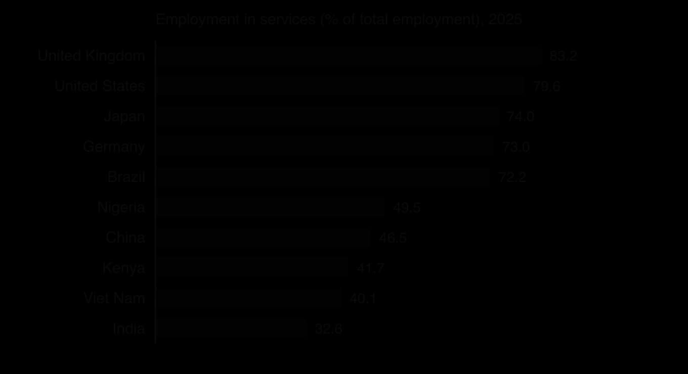
The three averages can be calculated on real data. The table gives the share of employment in services in ten countries in 2025.
Country | UK | USA | Japan | Germany | Brazil | Nigeria | China | Kenya | Viet Nam | India |
|---|---|---|---|---|---|---|---|---|---|---|
Employment in services (% of total) | 83.2 | 79.6 | 74.0 | 73.0 | 72.2 | 49.5 | 46.5 | 41.7 | 40.1 | 32.6 |
Sources: International Labour Organization, ILOSTAT modelled estimates, via World Bank World Development Indicators (SL.SRV.EMPL.ZS), retrieved October 2026.
The bar chart shows the two groups that the averages hide. It is sorted from highest to lowest, which makes the ranking and the gap easy to see, and its bars start from zero so that their lengths are proportional to the values.
Average | Advantages | Limitations | Best used for |
|---|---|---|---|
Mean | Uses every value; can be used in further calculations (totals, forecasts) | Distorted by extreme values (outliers); may not be an actual value (2.4 children) | Data without extreme values: average order value, average daily output |
Median | Not affected by extreme values; shows the “typical” middle case | Ignores the size of most values; cannot be combined easily across groups | Skewed data: pay, house prices, income, delivery times |
Mode | Easy to find; the only average for categorical data; always an actual value | May not exist or may be several; ignores most of the data | Stock and product decisions: most popular size, flavour, model |
An outlier is a value far above or below most of the other values in a data set. It may be a genuine but unusual value (one very large customer order) or an error in the data (a weight entered in grams instead of kilograms). Outliers should be checked before they are used: a genuine outlier is part of the picture, while an error should be corrected or removed.
When a few values are much larger than the rest, the distribution is positively skewed: most values are bunched at the low end and a long tail stretches to the right. Pay, wealth, house prices and the sizes of firms are all positively skewed. In a positively skewed distribution the mode is lowest, the median is in the middle and the mean is highest, because the mean is pulled towards the long tail.
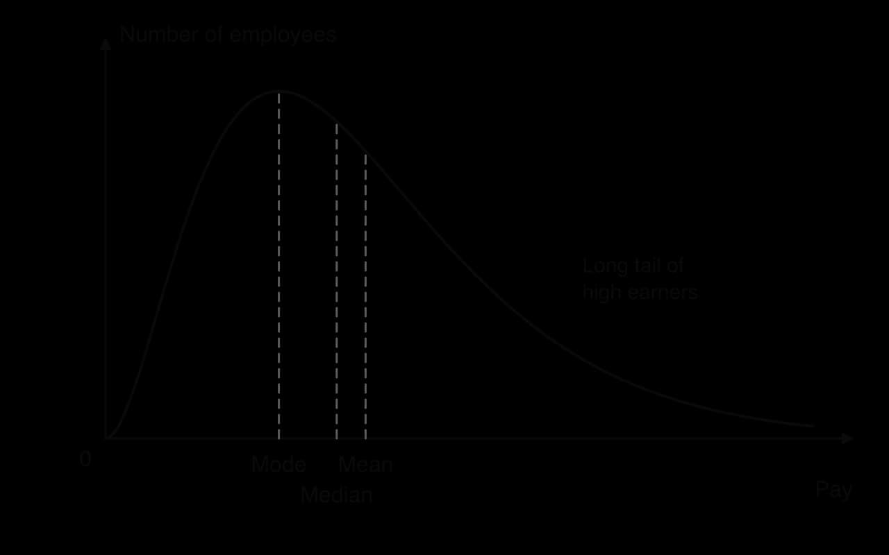
In a symmetrical distribution, such as the weights of packets filled by a well-adjusted machine, the mean, median and mode are equal. The further apart the mean and the median are, the more skewed the data. Comparing the two is therefore a quick test of skewness: a mean well above the median shows a long tail of high values.
Two data sets can have the same average but very different spreads. A café that serves between 48 and 52 customers every lunchtime and one that serves between 20 and 80 have the same mean of 50, but the second is much harder to staff and stock. Measures of spread (dispersion) show how far the values are spread around the average.
The range is quick to calculate and easy to understand, but it depends only on the two most extreme values. A single outlier can make the range very large even when nearly all the values are close together.
Quartiles divide ordered data into four equal parts. The lower quartile (Q1) is the value below which a quarter of the data lie; the median (Q2) is the middle; the upper quartile (Q3) is the value below which three quarters of the data lie. The interquartile range (IQR) is the spread of the middle half of the data, so it ignores the extreme quarter at each end.
Because the quartiles mark the edges of the middle half of the data, the distance between them is a measure of spread that is not affected by outliers.
Percentiles extend the same idea to 100 parts. The 10th percentile is the value below which 10% of the data lie, and the 90th percentile the value below which 90% lie; the median is the 50th percentile and the quartiles are the 25th and 75th. Statistics offices and employers use percentiles to describe pay, because they show the whole distribution rather than one average.
A box plot (box-and-whisker diagram) shows the quartiles at a glance: a box from Q1 to Q3 with a line at the median, and whiskers out to the extremes or to chosen percentiles. Two box plots side by side compare both the averages and the spreads of two groups, such as the delivery times of two suppliers.
The standard deviation measures how far, on average, the values in a data set lie from their mean. A small standard deviation means the values are clustered tightly around the mean; a large one means they are widely spread. Unlike the range and the IQR, it uses every value in the data set.
The formula works in four steps: find the mean; find how far each value is from the mean (its deviation); square each deviation, so that values below the mean do not cancel out values above it; then average the squared deviations and take the square root to return to the original units. Calculators and spreadsheets do this in one step, but working it through once on a small data set shows what the figure means.
The standard deviation is most useful for comparing the consistency of two or more data sets measured in the same units: the delivery times of two couriers, the weights of products from two machines, or the monthly sales of two branches. In quality control, a rising standard deviation in the weights of packets from a filling machine is an early warning that the machine needs adjustment, even if the mean weight is still correct.
 YouTube
A well-chosen chart shows a pattern faster than a table. The type of chart should match the question it answers: comparing categories, showing parts of a whole, showing change over time, or showing a relationship between two variables.
Bar charts compare values across categories: sales by region, market share by brand, scores by country. Vertical bars are often called a column chart. Grouped bars compare two or more series for each category, such as this year’s and last year’s sales for each product; stacked bars show how each total is made up. The services employment chart is a horizontal bar chart, which suits long category names.
The value axis starts at zero, so that bar lengths are proportional to the values.
Bars are the same width with equal gaps, and are sorted by size when the categories have no natural order.
The chart has a title, labelled axes with units, and a source.
A pie chart shows how a whole is divided into parts: the shares of a market held by each competitor, the breakdown of costs, or the share of employment in each sector of an economy. Each sector’s angle is its share of the total multiplied by 360°.
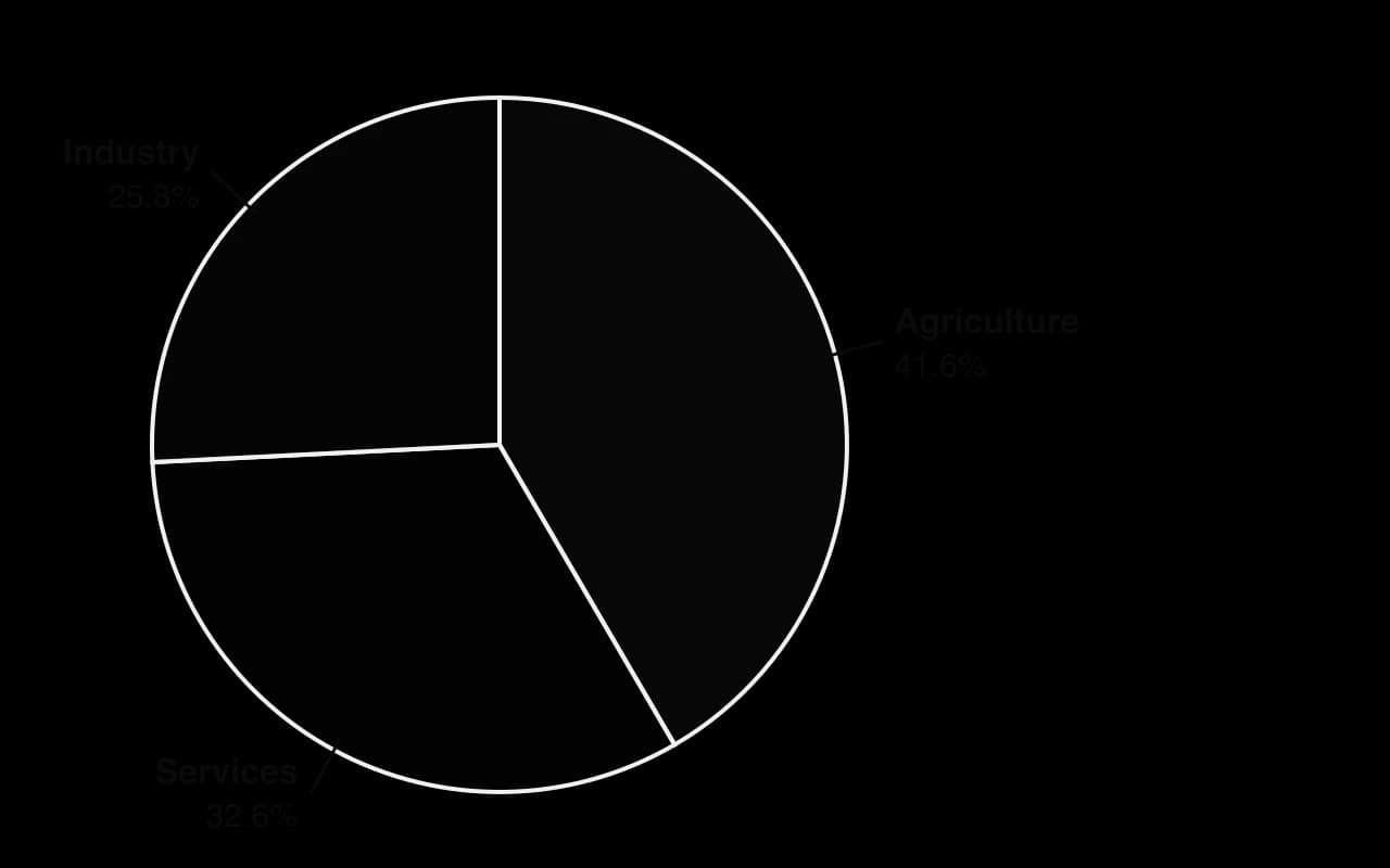
The pie chart works because there are only three parts that add up to a meaningful whole (100% of employment). Pie charts become hard to read with more than five or six sectors, or when the sectors are of similar size, because the eye judges angles less accurately than lengths. For comparing the same breakdown across several countries, a stacked bar chart is clearer.
A line graph plots values against time and joins the points, so it shows trends and seasonal patterns clearly; it is the standard chart for a time series such as monthly sales. Two or more lines on the same axes compare series over time, such as a firm’s sales against its competitors’. Line graphs are the basis of sales forecasting, in which a trend is drawn through past data and extended forward.
An infographic presents a few key statistics in a visual, easy-to-share form: a company’s annual results on one page, the findings of a customer survey, or a government’s summary of a new statistic. Businesses use them in annual reports, on social media, in recruitment campaigns and in internal communication, because they hold attention better than tables.
Because infographics simplify data, they have limitations. They usually show only selected figures, often without the sample size, the method or the spread of the data, and their design choices (icons scaled by area, bold colours on favourable figures) can exaggerate differences. They are useful for communicating a message, less so for analysing data or making decisions.
Purpose | Suitable chart | Example |
|---|---|---|
Compare values across categories | Bar (column) chart | Sales by region; market share by brand |
Show parts of a whole | Pie chart (few parts) or stacked bar | Shares of costs; market shares |
Show change over time | Line graph | Monthly sales; share price; labour turnover by year |
Show the spread of data | Box plot or histogram | Pay distribution; delivery times |
Show the relationship between two variables | Scatter diagram | Advertising spending against sales |
Communicate key figures to a general audience | Infographic | Annual results summary; survey highlights |
A chart can mislead even when every number in it is correct. The most common technique is a truncated axis: starting the vertical axis just below the lowest value makes a small change look large. The two charts show the same data, the share of UK employment in services from 2019 to 2025.

Every value in chart A is accurate and its axis is labelled, but the chart invites the reader to see a dramatic change. A truncated axis can be justified on a line graph when the point is to show small year-to-year movements, provided the break is clear; it should never be used on a bar chart, where readers compare bar lengths. Other common techniques include:
Choosing the period that tells the desired story, such as starting a chart of share prices at their lowest point.
Unequal intervals on the time axis, so that a slow change looks fast.
Three-dimensional or tilted pie charts, which make sectors at the front look larger.
Pictograms scaled by height and width, so that a figure twice as tall has four times the area.
Two vertical axes with different scales, which can make any two series appear to move together.
Choosing the average: quoting the mean pay of a group with a few very high earners, or the median when the mean would look better.
Leaving out the sample size, so that “80% of customers recommend us” may be based on 10 people.
 YouTube
Presenting data honestly is an ethical issue for businesses. Investors, employees and customers make decisions from the charts in annual reports, pay reports and advertisements. The UK Advertising Code, applied by the Advertising Standards Authority, states that marketing communications must not materially mislead, and statistics and comparisons in advertisements are judged by that rule. A firm found to be presenting data selectively loses credibility with all its stakeholders.
Descriptive statistics are used in every function of a business and with most of the other tools in the course.
Area | Typical use | Example |
|---|---|---|
Human resource management | Pay levels and pay gaps; absence; labour turnover; appraisal scores | Median and mean pay by grade; the spread of pay between the lowest- and highest-paid |
Finance and accounts | Average costs and revenues; comparing ratios with industry averages | Mean monthly cash inflow; standard deviation of monthly sales for a cash flow forecast |
Marketing | Market research results; customer satisfaction scores; sales by segment | The mode of preferred product features; the mean and spread of satisfaction ratings |
Operations management | Quality control; delivery times; productivity | Standard deviation of product weights; mean and range of lead times from suppliers |
Pay reporting in Great Britain shows how the choice of statistic matters. Since April 2017, every private and voluntary sector employer with 250 or more employees has had to publish its mean and median gender pay gaps in hourly pay and in bonus pay, and the proportion of men and women in each quarter of its pay distribution. Because both averages and the quartiles must be published, a firm cannot report only the figure that shows it in the best light.
Sources: UK Government, Gender pay gap reporting: guidance for employers, gov.uk, updated May 2026; The Equality Act 2010 (Gender Pay Gap Information) Regulations 2017 (SI 2017/172).
In market research, descriptive statistics summarise survey results: the mode shows the most popular answer to a multiple-choice question, the mean and standard deviation summarise a rating scale, and a bar or pie chart presents the results to managers. In operations, the mean and standard deviation of supplier lead time help set the buffer stock a business needs.
Descriptive statistics turn large amounts of data into information that managers can act on. They are quick to calculate with a spreadsheet, easy to communicate, and allow comparisons between products, branches, periods and competitors. Used together, an average, a measure of spread and a chart give a much fuller picture than any one of them.
Their limitations come from the data and from the choices made in presenting them:
The quality of the data. Statistics are only as reliable as the data behind them. A small or biased sample, out-of-date figures or errors in recording produce precise-looking but misleading results.
A single figure hides detail. An average says nothing about spread, and neither says anything about the shape of the distribution or the groups within it, as the services employment data show.
Subjective choices. The analyst chooses which average to report, which period to show, how to group the data and how to draw the chart, and each choice can change the impression given.
Description, not explanation. Descriptive statistics show what happened, not why. Explaining a pattern needs further analysis, such as simple linear regression or qualitative research, and judgment.
Qualitative factors are left out. Employee morale, brand image and customer loyalty are hard to reduce to a number, yet they may matter more to a decision than the figures do.
The usefulness of descriptive statistics therefore depends on the quality and size of the data set, on whether the measures chosen suit the shape of the data (the median and IQR for skewed data, the mean and standard deviation for symmetrical data), and on whether the people using them understand what they leave out. A decision supported by well-chosen statistics, presented honestly and combined with qualitative judgment, is better informed than one based on intuition alone.
The UK’s Office for National Statistics (ONS) measures pay through the Annual Survey of Hours and Earnings (ASHE), which collects pay data from employers for a 1% sample of employee jobs, identified from tax records; the 2025 survey had an achieved sample of 174,000 jobs. Its results are used by employers to benchmark pay, by the government to set policy, and by trade unions in pay negotiations.
In April 2025 the median gross annual pay of full-time employees who had been in the same job for at least a year was £39,039, while the mean was £48,512, about 24% higher. Weekly figures show the same gap: median full-time weekly pay was £766.60 and mean weekly pay £920.80. Both are correct measures of the “average” salary, but they describe different things.
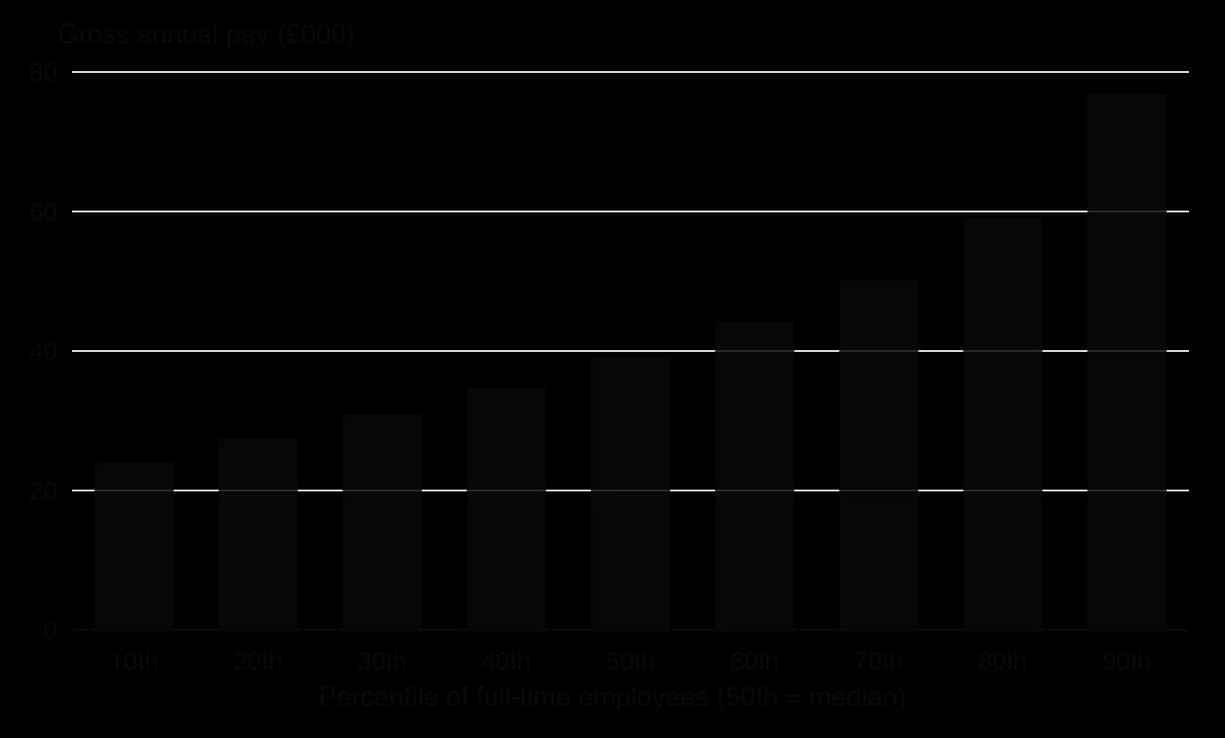
The chart shows why the mean is so much higher than the median. Pay rises slowly through the lower and middle percentiles and then much faster at the top: the 90th percentile (£76,903) is 3.2 times the 10th (£23,990). Pay is positively skewed, with a long tail of high earners above the 90th percentile that the chart cannot even show. Those high salaries raise the mean, while the median, the pay of the employee in the middle, is unaffected by them.
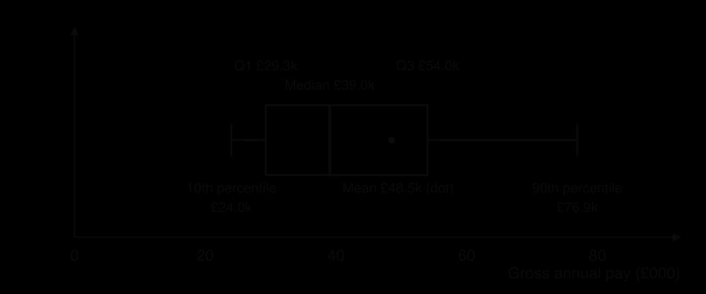
The box plot summarises the distribution. The lower quartile was £29,262 and the upper quartile £54,009, so the interquartile range was £24,747: the middle half of full-time employees earned within a band about £25,000 wide. The distance from the median to the upper quartile (£14,970) is greater than the distance from the lower quartile to the median (£9,777), another sign of skew.
Statistic, full-time employees, UK, April 2025 | Gross annual pay |
|---|---|
10th percentile | £23,990 |
Lower quartile (25th percentile) | £29,262 |
Median (50th percentile) | £39,039 |
Mean | £48,512 |
Upper quartile (75th percentile) | £54,009 |
90th percentile | £76,903 |
Interquartile range | £24,747 |
For a business, the choice of statistic has practical consequences. An employer benchmarking a job against “average pay” would overpay by using the mean for a typical role and should compare its pay with the percentile that matches the job’s level. A retailer designing products for the typical household would look at median incomes. A trade union seeking a pay rise may quote the growth of the median, which rose 4.3% in the year, while the mean rose 6.0%, a sign that pay at the top grew faster.
The data have limits. They cover employee jobs only, not the self-employed; they measure pay per job, so a person with two jobs appears twice; they are national figures that hide wide differences between regions, industries and occupations; and the 2025 figures are provisional and may be revised when the final results are published.
Sources: Office for National Statistics, Employee earnings in the UK: 2025 (23 October 2025) and Annual Survey of Hours and Earnings 2025 provisional, Tables 1.1a and 1.7a, retrieved October 2026.
Explain why the mean annual pay of full-time employees in the UK is higher than the median.
Calculate the range between the 10th and 90th percentiles and comment on what it shows.
Analyse which measure of average pay a UK supermarket should use when setting the pay of its store staff.
Descriptive statistics appear mainly in Paper 2, where stimulus material often includes tables, bar and pie charts or infographics, and in the internal assessment, where you summarise data from your supporting documents. Questions ask you to calculate an average or a measure of spread, construct or complete a chart, and comment on what the data show and how reliable they are.
Short calculation questions use small data sets from the stimulus.
Descriptive statistics summarise data with averages, measures of spread and charts; they describe data but do not explain them.
The mean uses every value but is distorted by outliers; the median is the middle value and suits skewed data; the mode is the most common value and suits categorical data and stock decisions.
In positively skewed data, such as pay, the mean is greater than the median, which is greater than the mode.
The range, interquartile range (Q3 − Q1) and standard deviation measure spread; the IQR ignores extremes and the standard deviation uses every value.
Bar charts compare categories, pie charts show parts of a whole, line graphs show change over time and infographics communicate key figures to a general audience.
Charts mislead through truncated axes, chosen periods, distorted areas and selective averages; honest presentation is an ethical responsibility.
Statistics are only as good as the data behind them and should be combined with qualitative judgment.
I can define descriptive statistics and explain why businesses use them.
I can calculate the mean, median and mode and explain which average suits a given data set.
I can explain why the mean is greater than the median in positively skewed data such as pay.
I can calculate the range, quartiles and interquartile range of a small data set.
I can calculate and interpret the standard deviation of a small data set.
I can construct a pie chart by calculating the angle of each sector, and draw a labelled bar chart.
I can choose an appropriate chart and identify ways in which a chart may mislead.
I can apply descriptive statistics to a decision in HR, finance, marketing or operations.
Award [1] for each correct mean with working. Award [1] in total if both answers are correct but no working is shown. Accept 5.1 and 7.5.
Using Table 1, explain how the leadership styles of the two principals may account for the differences in the survey results.
4 marks
Mr Tan (autocratic): decisions are made without consulting teachers, which explains the very low score for “My views are considered” (3.9) and for feeling trusted (4.8). Professional teachers may feel their expertise is ignored, lowering enjoyment (5.2) and willingness to recommend the school (5.5).
Dr Nair (democratic): working groups involve teachers in decisions, so views are considered (8.1) and teachers feel trusted (7.9). Participation can meet esteem needs and raise job satisfaction (7.4).
The smallest gap is for “I understand what is expected of me” (6.1 vs 6.8): clear instructions under an autocratic style help clarity, so this is one area where Mr Tan’s style is less of a disadvantage.
Other factors may also explain the differences (pay, workload, location, student behaviour), so leadership style may not be the only cause.
Award [1]–[2] for a limited explanation that links the results to leadership style with little use of the data.
Award [3]–[4] for an explanation that refers to both styles and uses specific scores from Table 1. Accept OFR from (a).
Hollenstein Components
Hollenstein Components (HC) has manufactured metal parts for car makers in Kalindor, a country in central Europe, since 1978. It employs 640 people at a factory in Brenholm, a former steel town. HC’s managing director, Jana Kovář, is preparing a five-year plan and has collected the national employment data shown in Table 1.
Table 1: Employment by sector in Kalindor (000s of workers)
Sector | 2005 | 2025 |
|---|---|---|
Primary | 1 800 | 900 |
Secondary | 2 400 | 1 950 |
Tertiary | 3 300 | 4 650 |
Quaternary | 500 | 1 500 |
Total | 8 000 | 9 000 |
Jana has also learned that two car makers that buy from HC plan to move some assembly to lower-cost countries, and that a software company has opened a research centre in Brenholm, recruiting engineers from HC.
Using Table 1, calculate the percentage change in secondary sector employment in Kalindor between 2005 and 2025 (show all your working).
2 marks
Using Table 1, calculate the quaternary sector’s share of total employment in Kalindor in 2025 (show all your working).
2 marks
Using Table 1, explain the sectoral change that has taken place in Kalindor.
4 marks
Analyse the implications for HC of the changes in Kalindor’s economy.
6 marks
Puerto Lirio is a coastal town in southern Chile. Its council wants to encourage more people to start businesses in the town and has published the employment data in Table 1. Fishing has declined because of quotas, while tourism has grown since a new airport opened in 2018. A growing number of people now work remotely from Puerto Lirio for software and design companies based in Santiago.
Table 1: Employment by sector in Puerto Lirio
Sector | 2010 | 2025 |
|---|---|---|
Primary | 4 200 | 2 700 |
Secondary | 2 100 | 1 800 |
Tertiary | 3 300 | 6 300 |
Quaternary | 400 | 1 200 |
Total | 10 000 | 12 000 |
The council plans to show the 2025 data as a pie chart. Calculate the angle of the segment for the tertiary sector (show all your working).
2 marks
Using Table 1, explain two opportunities for people thinking of starting a business in Puerto Lirio.
4 marks