Construct decision trees with decision nodes, chance nodes and outcomes, calculate expected values step by step, prune the rejected options and evaluate the tree as a basis for a risky decision.
Each is in the Business glossary, with every other term in the subject.
A point in a decision tree, drawn as a circle, from which two or more possible outcomes follow that are outside the decision maker's control, each with a probability.
A point in a decision tree, drawn as a square, at which the decision maker chooses between two or more options.
A diagram that sets out the options available in a decision, the possible outcomes of each with their probabilities and financial results, so that the expected value of each option can be calculated and compared.
The weighted average financial result of an option, found by multiplying the value of each possible outcome by its probability and adding the results.
The financial result of a particular outcome at the end of a branch of a decision tree, such as the revenue or profit it would bring, before the cost of the option is deducted.
The likelihood that an outcome will occur, expressed as a number from 0 (impossible) to 1 (certain); the probabilities of all outcomes at a chance node add up to 1.
Marking the options rejected at a decision node of a decision tree with two short parallel lines across their branches, leaving the option with the highest net gain (expected value minus cost).
Describe the parts of a decision tree: decision nodes, chance nodes, branches, probabilities and payoffs.
Explain why the probabilities at each chance node add up to 1, and where business probabilities come from.
Calculate the expected value of an option, step by step, and the net gain after its cost.
Construct a decision tree from data for a decision with two or three options and prune the rejected options.
Construct and solve a decision tree in which a second decision follows a chance outcome.
Explain how risk attitudes and qualitative factors can lead managers to choose an option that does not have the highest expected value.
Explain the advantages and limitations of decision trees, including the reliability of the estimates.
A decision tree is a diagram that sets out the options in a decision, the possible outcomes of each option, how likely each outcome is and what it is worth, so that the options can be compared in money terms. It suits decisions whose results are uncertain, such as launching a product, choosing a location, investing in research or deciding whether to go to court.
Decision trees help managers deal with change and uncertainty in a structured way. They also raise questions of ethics: a tree values outcomes only in money, so a decision about a product’s safety or a factory closure can look simple on the tree while affecting people in ways that the numbers leave out.
35 exam-style questions on this subtopic, written in the style of the IB papers. The first has its markscheme open. Counted on
Zhou Precision Components
Zhou Precision Components (ZPC) is a public limited company in Dongguan, China, that makes aluminium housings for laptops and tablets. About 60 % of its output is sold to two electronics brands that assemble products for export to Europe and the United States. ZPC employs 1 400 production workers, 300 of whom are on temporary contracts.
ZPC’s planning director, Zhou Lin, has prepared three scenarios for sales revenue in 2026 (Table 1). The pessimistic scenario assumes that new import tariffs on Chinese electronics are introduced, which would lead ZPC’s two main customers to move some assembly to Vietnam. Zhou Lin has estimated the probability of each scenario from discussions with customers and industry analysts.
The chief executive wants a single sales forecast so that ZPC can set its production plan, decide how many temporary contracts to renew and agree a budget with its bank. Some board members argue that, in such an uncertain trading environment, sales forecasting is “guesswork dressed up as science”.
Table 1: ZPC’s sales revenue scenarios for 2026
Scenario | Probability | Sales revenue (¥m) |
|---|---|---|
Optimistic | 0.25 | 480 |
Most likely | 0.55 | 400 |
Pessimistic | 0.20 | 260 |
In 2025 ZPC’s sales revenue was ¥410m.
Using Table 1, calculate the expected value of ZPC’s sales revenue for 2026 (show all your working).
The official deck for this part of the syllabus.
What is a decision tree?
What kind of decision is a decision tree suited to? Give three examples.
With a free account, Augment remembers where you stopped and what you have practiced.
Many business decisions have more than one possible result. A new product may sell well or badly; a new shop may attract many customers or few; a court case may be won or lost. The manager cannot control which result happens, but can choose the option. A decision tree separates the two: the choices the manager controls, and the outcomes that depend on chance.
A decision tree breaks a complicated decision into a sequence of simple ones. Building it requires the manager to list every option, to estimate how likely each outcome is and to put a value on it. The calculation then shows which option gives the highest average return, allowing for its risk and its cost. Decision trees are a quantitative tool, so they are used alongside qualitative judgement rather than instead of it.
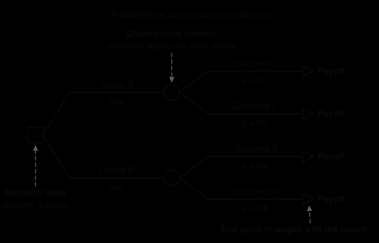
Decision trees use a standard set of symbols, drawn from left to right in the order in which events happen.
The diagram shows one decision between two options, A and B. Each option leads to a chance node with two possible outcomes. Each outcome has a probability and ends in a payoff. The cost of each option is written on its branch, so that it can be subtracted later.
A decision node is drawn as a square. It marks a point at which the business chooses between options, for example “launch nationally” or “launch regionally”. Each branch leaving a decision node is an option, labelled with its name and its cost. No probabilities are written on these branches, because the manager chooses which one to take.
A chance node is drawn as a circle. It marks a point at which the result depends on events outside the business’s control, such as the level of demand, the weather or the decision of a regulator. Each branch leaving a chance node is a possible outcome, labelled with its name and its probability.
Each branch ends in an outcome, often marked with a small triangle. The value written at the end is the payoff: the financial result of that outcome, such as the revenue or profit it brings. In most trees the payoffs are written before the cost of the option is deducted, and the cost is subtracted once the expected value has been calculated. If the payoffs given already include the cost, nothing more is subtracted.
A probability measures how likely an outcome is, on a scale from 0 (impossible) to 1 (certain). A probability of 0.7 means that the outcome would happen about 7 times in every 10 similar situations. Probabilities can also be written as percentages (70%), but decision trees normally use decimals.
At every chance node, the outcomes listed must cover everything that can happen, and only one of them can happen. Their probabilities must therefore add up to exactly 1. If high demand has a probability of 0.6 and there are only two outcomes, low demand must have a probability of 1 − 0.6 = 0.4.
Past data: the share of previous product launches that succeeded, or the number of rainy days at a site in previous years.
Market research: a survey or a test launch suggests how likely high demand is.
Forecasts by specialists: weather services, economists and industry analysts publish probabilities. The UK Met Office, for example, explains that a 70% chance of rain means a 7 in 10 chance that rain will fall at some point in the period, a figure an outdoor event organiser can use directly.
Industry studies: in some industries, large studies of past projects give success rates for each stage, as in drug development.
Managers’ judgement: when no data exist, experienced managers estimate the probabilities, which makes them more subjective.
Sources: Met Office, “What does this forecast mean?” (accessed October 2026).
An option with uncertain outcomes does not have a single result. To compare options, the decision tree uses the expected value: the average result the option would give if the same decision were made many times, with each outcome weighted by its probability.
Once the expected value at a chance node is known, the cost of the option is subtracted to give the net gain (sometimes called the net expected value) of that option.
If high demand (probability 0.6) brings $900,000 and low demand (probability 0.4) brings $200,000, the expected value is 0.6 × $900,000 + 0.4 × $200,000 = $540,000 + $80,000 = $620,000. If the option costs $300,000, the net gain is $320,000.
Decision trees are drawn from left to right, in the order in which events happen, and then solved from right to left. Working backwards from the payoffs to the first decision is called rolling back the tree.
Draw the first decision as a square on the left, with one branch for each option. Label each branch with the option and its cost.
Add a chance node (circle) at the end of each option whose result is uncertain, and draw one branch for each possible outcome. An option with a certain result goes straight to its payoff.
Write the probability on each outcome branch and check that each set adds up to 1.
Write the payoff at the end of each branch.
Roll back: at each chance node, calculate the expected value and write it next to the circle.
Subtract the cost of each option from the expected value to find its net gain.
Choose the best option at the decision node (the highest net gain, or the lowest net cost), write its net gain next to the square and prune every other option.
Pruning means marking the rejected options with two short parallel lines across their branches (//). The pruned tree shows at a glance which option has been chosen and which have been rejected.
Trees can have any number of options, and an option may have a certain result with no chance node. The next example has three options, one of which is certain.
The expected values of the three options are close, and the options differ much more in their risk. The table compares the worst and best net results of each option with its net gain.
Option | Worst net result | Best net result | Net gain (EV − cost) |
|---|---|---|---|
Outdoors, no marquee | $30,000 | $120,000 | $93,000 |
Hire a marquee | $75,000 | $90,000 | $85,500 |
Move indoors | $90,000 | $90,000 | $90,000 |
Moving indoors gives up only $3,000 of expected value in exchange for removing all the risk. The marquee is never the best choice, because moving indoors does better if it rains ($90,000 against $75,000) and equally well if it is dry ($90,000 each). Organisers who could not survive a $30,000 result, for example because they must pay suppliers out of the event’s takings, would sensibly move indoors.
The recommendation depends on the 0.3 probability of rain. If the probability of rain is , the net gain from staying outdoors is dollars. This equals the certain $90,000 from moving indoors when . A forecast of 0.3 is only just below that level. If the forecast rose to 0.4, the outdoor option would fall to $84,000 and moving indoors would become the better choice.
Asking how far an estimate can change before the decision changes is a simple sensitivity check. When the decision changes with a small change in an uncertain probability, the tree gives only weak support to either option and qualitative factors deserve more weight.
The rule “choose the highest expected value” assumes that the decision maker cares only about the average result. Real managers also care about how bad the worst result could be. Their attitude to risk affects which option they prefer.
Attitude | Behaviour | Likely choice at the festival |
|---|---|---|
Risk-averse | Prefers a certain or safer result even at a lower expected value; typical of small firms, firms with weak cash flow and managers whose jobs depend on avoiding losses | Move indoors ($90,000 for certain) |
Risk-neutral | Chooses the highest expected value and ignores the spread of results; reasonable for large firms making many similar decisions, where good and bad outcomes average out | Outdoors (net gain $93,000) |
Risk-seeking | Is attracted by the chance of the largest result even at a lower expected value | Outdoors (chance of $120,000) |
The size of the decision compared with the business matters. A supermarket chain making hundreds of store decisions a year can behave in a risk-neutral way, because the average result is what it will in fact receive over time. A start-up whose survival depends on one product launch cannot, because a single bad outcome may close the business before the average has any meaning.
In some decisions a second choice follows a chance outcome. A business may first decide whether to carry out test marketing, and then, depending on the result, decide whether to launch. Such a tree has a decision node to the right of a chance node, and it is rolled back in the same way: from right to left, taking the best option at each later decision node before working out the expected value of the chance node before it.
The example shows why information has value. Market research, trials and pilots cost money, but they can change later decisions. A decision tree puts a money value on that flexibility: the test is worth buying only if the expected gain from making a better later decision exceeds the cost of the test.
Decision trees can be applied to any decision with clear options and uncertain, measurable outcomes.
Area | Example of a decision | Typical chance outcomes |
|---|---|---|
Marketing | National or regional launch; whether to test market; which advertising campaign to run | High, medium or low demand; competitor reaction |
Operations | Which location to choose; whether to build a larger factory or extend the current one | Demand at each site; construction delays |
Finance | Whether to invest in new machinery; compared with investment appraisal of each option | Sales growth; interest rate changes |
Human resources | Whether to recruit externally or train existing staff for a new role | Success of the appointment; staff leaving |
Strategy | Whether to enter a new market (an Ansoff matrix choice) or to settle or fight a legal case | Market acceptance; winning or losing in court |
A decision tree also works well with other tools. A SWOT analysis can identify the options worth putting on the tree; break-even analysis can supply payoffs; and a social enterprise can use a tree to compare ways of reaching its social objectives, with payoffs measured in people helped as well as in money.
Structure. The tree sets out every option and outcome in a clear, logical order, which makes complex decisions easier to understand and discuss.
Risk is made explicit. Managers must estimate how likely each outcome is, rather than assuming the best case.
Options are compared on the same basis. Expected values allow options with different costs and outcomes to be ranked.
Later decisions can be included. Multi-stage trees show the value of keeping options open, such as testing before launching.
Communication. The diagram is easy to present to a board, investors or other stakeholders, who can question each estimate.
Probabilities are estimates. They often come from judgement or from past data that may not apply to a new situation, so the result is only as good as these estimates.
Payoffs are forecasts. Revenues and costs years ahead are uncertain, especially for new products and in fast-changing markets.
Outcomes are simplified. Real demand can take any value, not just “high” or “low”, and a tree with only two or three outcomes may hide important possibilities.
Expected value ignores risk attitude. It treats a certain $90,000 and a gamble averaging $93,000 as nearly equal, which a business that cannot afford a bad outcome would not.
Qualitative factors are left out. Employee morale, ethics, brand reputation, the environment and the reaction of stakeholders are hard to put into money terms.
Time and bias. Gathering good data takes time, and managers can adjust estimates, consciously or not, to support the option they already prefer.
Timing of cash flows. Basic trees do not allow for when the payoffs arrive; a payoff in five years is treated the same as one received now.
A decision tree is most useful when the options are clear, the outcomes can be measured in money and the probabilities rest on good evidence, such as long runs of past data or industry studies. It is least useful for one-off strategic decisions in new markets, where probabilities are guesses and the most important consequences are qualitative. In every case the tree supports the decision. The expected values show the financial case, and managers then weigh the risk, the business’s objectives and finances, the reliability of the estimates and the effect on stakeholders before choosing.
 YouTube
Pharmaceutical and biotechnology companies make some of the largest and riskiest decisions in business. A new medicine is tested in a series of stages before a regulator can approve it: Phase I trials test safety in a small group of people, Phase II trials test whether the drug works, Phase III trials test it on large numbers of patients, and the company then files an application for approval (in the United States, a New Drug Application or Biologics License Application to the Food and Drug Administration). At the end of each stage the company makes a go or no-go decision: continue to the next, more expensive stage, or stop. This sequence of decisions and chance outcomes is a multi-stage decision tree.
An industry analysis published in 2021 covered 12,728 phase transitions in 9,704 development programmes at 1,779 companies over 2011–2020. It gives the probability that a drug moves successfully from each stage to the next.
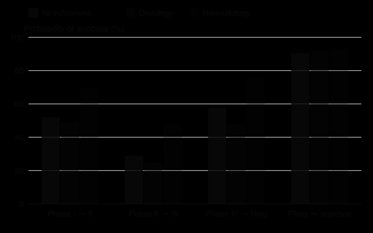
Stage transition (all disease areas) | Probability of success | Average time (years) |
|---|---|---|
Phase I → Phase II | 0.520 | 2.3 |
Phase II → Phase III | 0.289 | 3.6 |
Phase III → application filed | 0.578 | 3.3 |
Application → approval | 0.906 | 1.3 |
Phase I → approval (all four stages) | 0.079 | 10.5 |
The overall likelihood of approval from Phase I is the product of the four stage probabilities: 0.520 × 0.289 × 0.578 × 0.906 = 0.079, or 7.9%. Fewer than one drug in twelve that enters human trials reaches the market, and the average drug that does succeed takes 10.5 years. The probabilities in a drug development tree therefore rest on unusually good evidence, and they are low.
Sources: BIO, Informa Pharma Intelligence and QLS Advisors, Clinical Development Success Rates 2011–2020, February 2021.
The tree models a typical decision for a small biotechnology company whose drug has just passed Phase II. The probabilities are the real all-disease figures; the costs and payoffs are hypothetical. Funding Phase III costs $300 million. If Phase III succeeds (0.578) and the drug is approved (0.906), the company expects $1,000 million from sales. Alternatively, it can license the drug to a larger company for a certain $150 million.
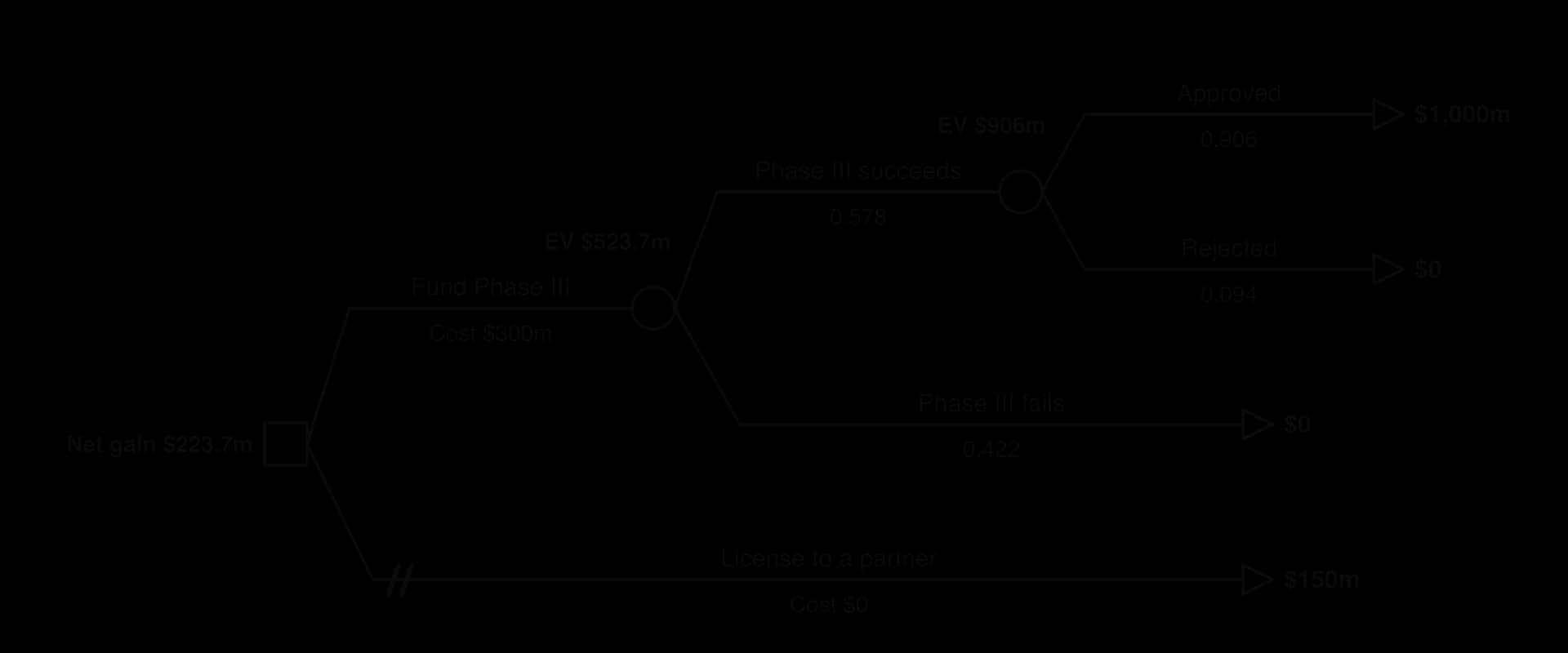
Rolling back the tree, the approval chance node is worth 0.906 × $1,000m = $906m, and the Phase III chance node 0.578 × $906m = $523.7m. After the $300m cost, the net gain from funding Phase III is $223.7m, higher than the $150m from licensing, so licensing is pruned. A risk-neutral company would fund the trial.
The tree also shows the risk. The probability of reaching approval is 0.578 × 0.906 = 0.524, so the company loses its whole $300m investment almost half the time (a probability of 0.476). A large pharmaceutical company with dozens of drugs in development can accept this, because successes and failures average out across its portfolio. A small company with one drug may not survive a failed Phase III, which explains why many small biotechnology firms license their drugs to larger partners even when the expected value of continuing alone is higher.
The probabilities vary by disease area. For oncology (cancer) drugs, the chance of passing Phase III is 0.477 and of approval after filing 0.920, so the probability of reaching the market from Phase III is 0.477 × 0.920 = 0.439. With the same payoffs, funding Phase III is worth 0.439 × $1,000m − $300m = $138.8m, less than the $150m from licensing, so the decision reverses. For haematology drugs (0.768 and 0.931) the net gain rises to $415.0m. With the same payoffs, the choice between funding and licensing therefore depends on the disease area.
Chance outcomes in drug trials can also come from unexpected events. In April 2025 Pfizer stopped developing danuglipron, an experimental weight-loss pill, after a trial participant suffered a liver injury. A probability of failure describes many projects on average and does not identify which project will fail or why.
The case shows both the strength and the limits of decision trees. Few industries have probabilities as well measured as drug development, which is why go or no-go decisions there are routinely analysed with trees. Even so, the payoffs (future sales of a drug that does not yet exist) are very uncertain, the money values leave out the ethics of which diseases receive research spending and the benefit to patients, and the tree ignores the 10.5 years over which the money is spent and received.
Sources: BIO, Informa Pharma Intelligence and QLS Advisors, Clinical Development Success Rates 2011–2020 (2021); CNBC, “Pfizer scraps daily weight loss pill after liver injury in one patient”, 14 April 2025 (via Wikipedia, Danuglipron).
Explain why the overall probability of approval from Phase I (0.079) is much lower than the probability of passing any single stage.
Analyse why a small biotechnology company might license its drug even when funding Phase III has the higher expected value.
Explain two limitations of using this decision tree to decide whether to fund Phase III.
Decision trees appear mainly in Paper 2, where you may be asked to construct a tree from data [4–6], calculate expected values [2–4], recommend an option, or explain the limitations of the tree [4]. They also make a good supporting tool in 10-mark answers and in the Paper 3 plan of action, where a tree can compare options for a social enterprise.
Construction and calculation questions usually come together, often followed by a question on limitations.
The extended response asks for a judgement that uses the tree and goes beyond it.
A decision tree shows the options in a decision (squares), the chance outcomes of each (circles), their probabilities and their payoffs.
The probabilities at each chance node add up to 1.
Expected value = the sum of (probability × payoff) for each outcome; net gain = expected value − cost of the option.
Trees are drawn left to right and solved right to left; rejected options are pruned with two short lines.
In a multi-stage tree, the best option at each later decision node is chosen before the chance node before it is valued.
Expected value is a long-run average; risk attitudes, the business’s finances and qualitative factors can justify a different choice.
The tree is only as reliable as its estimated probabilities and payoffs, so a sensitivity check strengthens any recommendation.
I can describe the parts of a decision tree and draw the correct symbol for each.
I can explain why the probabilities at a chance node add up to 1 and where business probabilities come from.
I can calculate expected values and net gains, showing every step.
I can construct and solve a decision tree with two or three options and prune the rejected options.
I can solve a multi-stage tree in which a decision follows a chance outcome.
I can explain how attitudes to risk and qualitative factors affect a decision.
I can explain the advantages and limitations of decision trees.
I can apply a decision tree to a real decision, such as funding a drug trial.
2 marks
= ¥392m
Award [1] for correct working and [1] for the correct answer. Award a maximum of [1] if the ¥ sign or “m” is missing.
Explain two ways in which a sales forecast could help ZPC plan its workforce.
4 marks
Answers may include:
Temporary contracts: the forecast indicates how many of the 300 temporary contracts to renew; the expected value of ¥392m (below 2025’s ¥410m) may suggest renewing fewer.
Recruitment and training lead times: if the optimistic scenario looks more likely, ZPC can recruit and train workers before orders arrive rather than paying overtime.
Shift patterns and overtime: production schedules for 1 400 workers can be set in advance, reducing idle time and overtime costs.
Avoiding redundancies: early warning of the pessimistic scenario allows ZPC to reduce staff through natural wastage rather than costly, demotivating redundancies.
Accept any other relevant way.
Mark as 2 + 2. For each way, award [1] for identifying it and [1] for explaining it in the context of ZPC.
Evaluate the usefulness of sales forecasting for ZPC in its current trading environment.
10 marks
Strengths/usefulness:
Forecasting provides a basis for the production plan, purchasing of aluminium and the budget the bank requires; without it, ZPC would plan blindly.
Scenario forecasting with probabilities recognises uncertainty rather than ignoring it; ZPC can prepare contingency plans for the pessimistic case (¥260m, a 36.59 % fall from 2025).
The expected value (¥392m) gives a single planning figure that weights each outcome by its likelihood.
Discussions with customers and analysts mean the forecast uses up-to-date market intelligence, not only past sales.
The forecast helps decide on temporary contracts, giving ZPC flexibility to match labour to demand.
Limitations:
Probabilities are subjective estimates; a small change in the probability of tariffs changes the expected value.
The expected value of ¥392m will not actually occur; ZPC will earn ¥480m, ¥400m or ¥260m (or something else), so planning for ¥392m may leave it with too much or too little capacity.
Political decisions on tariffs are hard to predict; dependence on two customers makes ZPC’s sales very sensitive.
Forecasting takes management time and may give false confidence (the board’s “guesswork” concern).
Technological change in laptops (new materials) may also affect demand and is not in the scenarios.
Possible conclusion: forecasting remains useful for ZPC, but as a range rather than a single number. ZPC should plan flexibly (temporary contracts, staged purchasing) and update forecasts as tariff news emerges. A well-supported judgement either way can achieve full marks.
Limitations of the stimulus: no information on ZPC’s costs, capacity or how past forecasts compared with actual sales; the basis for the probabilities is not explained.
Additional guidance:
Marks should be allocated according to the markbands below.
No use of Table 1 or the case data (scenario values, probabilities, ¥410m in 2025): maximum [4].
Only strengths or only limitations of forecasting: maximum [5].
No conclusion on how useful forecasting is for ZPC: usually maximum [6].
For [9]–[10], candidates should recognise limitations of the stimulus, such as the subjective probabilities.
Markbands (10-mark extended response, Papers 1 and 2)
Marks | Level descriptor |
|---|---|
0 | The response does not reach the standard described below. |
1–2 | Little understanding of what the question demands. Business management tools and theories are barely used, or are irrelevant or inaccurate. Little or no reference to the stimulus material. No arguments are made. |
3–4 | Some understanding of what the question demands. Some use of tools and theories, but mostly inaccurate or not relevant. Use of the stimulus is superficial, often no more than the name of the organisation or person. Arguments are mostly unsubstantiated. |
5–6 | Understands what the question demands but addresses it only partially. Some relevant, accurate use of tools and theories. Some relevant use of the stimulus beyond names, but it does not effectively support the argument. Arguments are substantiated but mostly one-sided. |
7–8 | Mostly addresses what the question demands. Mostly relevant, accurate use of tools and theories. The stimulus generally supports the argument, with some lapses in clarity or relevance. Arguments are substantiated and show some balance. |
9–10 | Clear focus on what the question demands. Relevant, accurate use of tools and theories. Relevant stimulus material is integrated effectively to support the argument. Arguments are substantiated and balanced, and the limitations of the case or stimulus material are explained. |
A response with no judgement or conclusion is unlikely to reach the top band of a discuss, evaluate, examine or recommend question.
Ankobra Cocoa Processors
Ankobra Cocoa Processors Ltd (ACP) grinds cocoa beans into cocoa butter and cocoa powder at a factory in Takoradi, Ghana, and sells them to chocolate manufacturers in Europe. Its factory is running at full capacity, and its managing director, Kwame Ofori, wants to double output to take advantage of growing demand and the Ghanaian government’s policy of processing more cocoa in the country instead of exporting raw beans.
Kwame is considering two options. Option A is to build a second grinding factory next to the existing one. Option B is to acquire Volta Grinders, a rival processor near Tema that has modern machinery but has lost money for two years because of poor management. ACP’s finance team has estimated the costs and the possible financial outcomes over the next eight years (Table 1).
Kwame knows that ACP’s managers have never run a second site, and that Volta Grinders’ 220 workers are unionised and worried about job losses.
Table 1: Estimated costs and outcomes of ACP’s growth options (GHS million)
Option | Cost | Outcome | Probability | Financial return |
|---|---|---|---|---|
A: build a second factory | 40 | Demand high | 0.6 | 90 |
Demand low | 0.4 | 50 | ||
B: acquire Volta Grinders | 55 | Integration successful | 0.7 | 110 |
Integration problems | 0.3 | 60 |
Distinguish between Option A and Option B as methods of growth.
2 marks
Using Table 1, calculate the net expected value of each option (show all your working).
4 marks
Using Table 1, your answers to (b) and other information in the case, recommend whether ACP should choose Option A or Option B.
10 marks
Ganyesa Catering (Pty) Ltd (GC)
GC is a South African company that cooks and delivers meals to schools and hospitals in North West Province. Its contracts are renewed every three years and profit margins are low. The directors want to grow and are considering two options:
Option A: provide the same meals to mining camps across the border in Botswana. This would cost R2.4 million.
Option B: launch a range of frozen ready meals for South African supermarkets. This would cost R1.5 million.
GC could also choose to do neither. The forecast outcomes are shown in Table 1.
Table 1: Forecast outcomes for GC’s options (total returns over three years, R million)
Option | Outcome | Probability | Returns (R million) |
|---|---|---|---|
A | Success | 0.6 | 6.0 |
A | Failure | 0.4 | 1.5 |
B | High demand | 0.5 | 4.8 |
B | Medium demand | 0.3 | 2.6 |
B | Low demand | 0.2 | 0.9 |
Using the Ansoff matrix, identify the growth strategy represented by Option A and by Option B.
2 marks
Using Table 1, construct a decision tree for GC’s options.
4 marks
Calculate the expected value of Option A and of Option B (show all your working).
4 marks
Using your answers to (a) and (c), explain which option GC should choose.
4 marks