C4.1 Populations and communities

A population is a group of organisms of the same species living in the same area at the same time. Members of a population interact with one another: they compete for food, water and space, they may cooperate, and above all they normally breed with one another. Interbreeding is what holds a population together as a unit, because genes pass between its members in every generation.

A species is often split into several populations. Two groups of the same species that live in separate places, such as brown trout (Salmo trutta) in two lakes with no stream connecting them, do not normally interbreed even though they could if they met. Biologists use this reproductive isolation to decide where one population ends and the next begins. Populations separated in this way are usually geographically separated: by a mountain range, a stretch of sea, or simply distance.

The boundaries of a population are not always sharp. A population of a sedentary snail in one hedgerow may be very local, whereas a population of a migratory bird may span a continent. Ecologists therefore define the area of a population for a particular study and treat the organisms inside it as one breeding group.

Estimating population size by random sampling

Why populations are estimated rather than counted

Counting every individual in a population is rarely possible. The organisms may be too numerous (the grass plants in a meadow), too small (soil invertebrates), hidden (burrowing animals), constantly moving, or spread over too large an area. A complete count would also often disturb or damage the habitat. Ecologists therefore count the organisms in samples and use the counts to estimate the size of the whole population.

For an estimate to be valid, the samples must be representative of the whole area. Random sampling achieves this: every individual, or every part of the area, has an equal chance of being included. If samples are chosen by eye, the person sampling tends to pick places where the organisms are easy to see or seem common, and the estimate is biased.

Sampling error

Even a perfectly random sample is unlikely to give exactly the true population size. By chance, some samples contain more organisms than average and others fewer. The difference between an estimate and the true value is called sampling error. Sampling error is an unavoidable consequence of measuring part of a population instead of all of it, and it is different from a mistake in method.

Sampling error can be reduced but never removed. Taking more samples, or larger samples, makes the estimate more reliable, because chance high and low counts tend to cancel out. Scientists also report how variable their samples were, so that readers can judge how much confidence to place in an estimate. This is an important idea in the nature of science: a measured value is always an estimate with some uncertainty attached.

Random quadrat sampling for sessile organisms

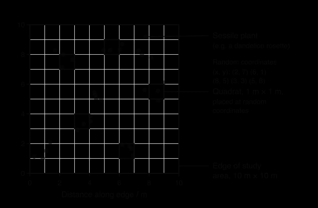
A quadrat is a square frame of known area, such as 0.25 m² (50 cm × 50 cm) or 1 m², placed on the ground to mark out a sample area. Quadrats are suitable for sessile organisms, which stay fixed in one place: plants, and sessile animals such as barnacles and mussels on a rocky shore. Limpets move only a short distance when the tide is in and return to the same spot, so they are also sampled with quadrats. Quadrats are not suitable for motile animals, which would move into or out of the frame while it is being placed.

Quadrats are positioned at random using coordinates. The method is as follows:

1. Mark out the study area, for example a 10 m × 10 m square, with two tape measures along adjacent edges as axes.

2. Generate pairs of random numbers (with a calculator, spreadsheet or random number table) to use as x and y coordinates.

3. Place the corner of the quadrat at each coordinate in turn.

4. Count the individuals of the species inside each quadrat. Decide a rule in advance for individuals lying across the edge, for example count those on two sides but not on the other two.

5. Repeat for enough quadrats that the mean count stops changing much as more are added (often 10–20 or more).

The population size is estimated from the mean number of individuals per quadrat and the total area:

Standard deviation of the mean count

Quadrat counts vary because organisms are not spread evenly. The standard deviation (SD) measures this spread: how far the individual counts typically lie from the mean. A small SD means the counts are similar to each other, so the mean is a good summary and the organisms are fairly evenly distributed. A large SD means the counts vary widely, which usually shows that the organisms are clumped, and the estimate of population size is less reliable.

Standard deviation is calculated with a calculator or spreadsheet (for example the STDEV function), so the formula does not have to be memorised. Reporting it alongside the mean, as mean ± SD, shows how much confidence to place in the estimate.

Capture–mark–release–recapture for motile animals

Animals that move around, such as beetles, woodlice, snails, small mammals and fish, cannot be counted in quadrats. Their population size is estimated by capture–mark–release–recapture. A sample is caught and marked, released to mix back into the population, and then a second sample is caught some time later. The proportion of marked animals in the second sample is used to estimate the size of the whole population.

1. Capture as many individuals as possible in a set time, using a method suited to the species (pitfall traps for ground beetles, Longworth traps for small mammals, nets for fish).

2. Mark each one in a way that does not harm it or change its behaviour, such as a small dot of non-toxic paint on the shell of a snail or under the wing case of a beetle. Count them: this number is M.

3. Release them where they were caught and leave enough time for them to mix randomly with the rest of the population.

4. Capture a second sample in the same way and count the total number caught (n) and the number of these that are marked (m).

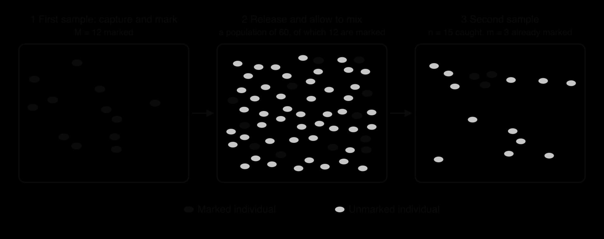
The method rests on a simple proportion. If the marked animals have mixed evenly, the fraction of the second sample that is marked equals the fraction of the whole population that is marked:

This is the Lincoln index, where N is the estimated population size, M the number caught and marked in the first sample, n the total number caught in the second sample and m the number of marked individuals in the second sample.

Assumptions of the Lincoln index

The Lincoln index gives a valid estimate only if several assumptions hold. Each one, if broken, biases the estimate in a predictable direction:

To meet these assumptions, ecologists choose a short interval between samples (long enough to allow mixing but too short for many births or deaths), use marks that are small and durable, and release animals exactly where they were caught.

Carrying capacity and competition for limited resources

Every organism needs resources to survive and reproduce. Animals need food, water, space, shelter and sites for nests or burrows; plants need light, water, mineral nutrients such as nitrate and phosphate, and space for roots and leaves. When resources are plentiful, a population grows. As it grows, each individual gets a smaller share of the resources, until the environment cannot support any more individuals.

The carrying capacity of an environment is the maximum population size of a species that it can support indefinitely. It is set by whichever resource runs short first, the limiting factor. For seabirds on a cliff it may be nesting ledges; for trees in a forest it is often light; for herbivores on an island it is usually food.

As a population approaches carrying capacity, individuals compete more intensely for limited resources. Those that obtain enough resources survive and breed; those that do not die or fail to reproduce. Carrying capacity is not fixed: it changes when resources change, for example falling in a drought or rising when a new food source becomes available.

• Food limits many animal populations, for example herbivores on islands with no predators.

• Water limits plant and animal populations in deserts and in dry seasons.

• Space and territory limit territorial animals such as European robins (Erithacus rubecula).

• Light limits plants in dense vegetation, such as seedlings on a forest floor.

• Nesting sites limit hole-nesting birds and cliff-nesting seabirds.

• Mineral nutrients such as nitrate and phosphate limit plants and algae, especially in nutrient-poor soils and lakes.

Negative feedback control of population size

Factors that change the size of a population are of two kinds. A density-dependent factor has an effect that becomes stronger as population density increases. A density-independent factor affects a population to the same extent whatever its density.

Density-dependent factors act by negative feedback. When a population rises above carrying capacity, their effects increase, so the death rate rises or the birth rate falls and the population shrinks. When the population falls below carrying capacity, their effects weaken, so the population grows again. The result is that the population is pushed back towards carrying capacity from either direction. The three main density-dependent factors are:

• Competition for resources. In a dense population each individual gets less food, water or space, so fewer survive and those that do produce fewer offspring.

• Predation. A dense prey population is easier for predators to find, and predators may switch to it or breed more successfully, so a larger proportion of the prey is eaten.

• Pathogens and pests. Infectious diseases and parasites spread faster when hosts are close together and meet often, so a larger proportion of a dense population becomes infected.

Density-independent factors include weather events such as frosts, droughts, floods and storms, and natural disasters such as fires and volcanic eruptions. A severe frost kills a similar proportion of insects whether there are few or many. These factors cause sudden fluctuations in population size but do not, by themselves, return the population to a set level.

Population growth curves

Exponential growth

When a few individuals colonise an environment with plentiful resources and no predators or diseases, the population grows by exponential growth. Each individual produces offspring, and those offspring soon breed too, so the number added in each time interval is proportional to the number already present. The population doubles in a fixed time, giving a curve that rises ever more steeply: the J-shaped curve.

Exponential growth happens in the initial phase of colonisation because resources are abundant, there is no competition yet, and predators and pathogens are absent or rare. The birth rate is therefore much higher than the death rate. No real population can grow exponentially for long, because resources eventually become limiting.

Sigmoid growth

In most populations, growth slows as resources become limited and density-dependent factors take effect. The resulting S-shaped curve is the sigmoid growth curve, which has three phases:

1. Exponential phase. Resources are plentiful and limiting factors are absent, so the birth rate greatly exceeds the death rate and the population increases rapidly.

2. Transitional phase. Resources start to become limiting. Competition, predation and disease increase, so the birth rate falls and the death rate rises. The population still grows, but more slowly.

3. Plateau phase. The birth rate equals the death rate (or births plus immigration equal deaths plus emigration), so the population stops growing and fluctuates around the carrying capacity.

The graph of the two models shows that they are identical while the population is small, because resources are not yet limiting. The difference between them grows as the population approaches carrying capacity. At the plateau, individuals are still being born and dying; the population is constant only because the two rates are equal.

Growth curves as models

The exponential and sigmoid curves are idealised graphical models. Real populations rarely follow them exactly: they overshoot carrying capacity, fluctuate around it, or crash. A model is still useful because it identifies the processes that matter (birth rate, death rate, limiting resources) and gives a baseline against which real data can be compared. When real data depart from a model, the difference points to factors the model leaves out, such as time delays or changes in the environment.

Testing for exponential growth with a logarithmic scale

On an ordinary (linear) scale, exponential growth gives a curve, and it is hard to tell by eye whether a curve is exactly exponential. Plotting population size on a logarithmic scale solves this. Each equal step on a log scale represents multiplication by the same factor (1, 10, 100, 1000…). Because exponential growth multiplies the population by the same factor in each time interval, it gives a straight line when population size is plotted on a log scale against time on a linear scale.

If the points on a log plot lie on a straight line, growth is exponential, and the gradient gives the growth rate. If the line bends downwards, growth is slowing, as it does in the transitional phase of the sigmoid curve. In practice, log₁₀ of each population size is calculated and plotted on ordinary graph paper, or a spreadsheet axis is set to a log scale.

Case study: the reindeer of St Matthew Island

St Matthew Island is a small, remote island in the Bering Sea, between Alaska and Siberia. In 1944 the US Coast Guard released 29 reindeer (Rangifer tarandus) there as an emergency food source for the men of a radio navigation station. The island had a thick mat of lichens, the main winter food of reindeer, and no wolves or other predators. The station was soon abandoned, leaving the reindeer to grow without hunting.

With abundant food and no predators, the population grew rapidly. Biologists counted about 1,350 reindeer in 1957 and about 6,000 in the summer of 1963. By then the lichen had been grazed down so heavily that much of the island was almost bare of it. In the severe winter of 1963–64, with deep snow covering the little food that remained, most of the herd starved. When biologists returned in 1966 they found only 42 reindeer: 41 females and one male, which was infertile, so the herd could not recover and later died out.

Source: Klein, D. R., Journal of Wildlife Management 32: 350–367, 1968.

The St Matthew reindeer show the early part of population growth very clearly. For 19 years there was no limiting factor: food was abundant, there were no predators, and the population grew in a roughly exponential way. The population did not level off at a plateau as the sigmoid model predicts. Lichen grows very slowly, so the effect of grazing on the food supply showed up years after the damage was done. By the time food became limiting, the population had overshot the carrying capacity by a wide margin.

The crash combined a density-dependent factor with a density-independent one. Shortage of food was density-dependent: the more reindeer there were, the less lichen each one had. The severe winter was density-independent, but it struck a population that was already starving. Overgrazing had also lowered the carrying capacity of the island itself, so it could no longer support even the number of reindeer it once could.

The log plot of the reindeer growth phase makes the comparison with the exponential model easy. The three points lie close to a single straight line, with the 1957 point slightly above it, which matches the slightly faster growth calculated for the earlier period.

Modelling sigmoid growth in the laboratory

Population growth can be followed in the laboratory with organisms that reproduce quickly in a small space. Two organisms are especially suitable. Yeast (Saccharomyces cerevisiae) is a single-celled fungus that reproduces by budding every few hours in a sugar solution. Common duckweed (Lemna minor) is a tiny floating plant whose leaf-like fronds bud off new fronds every few days.

Method for duckweed

1. Fill several identical containers with the same volume of pond water or a dilute mineral nutrient solution.

2. Place the same number of fronds (for example 10) in each container, and keep them at the same temperature and light intensity.

3. Every two or three days, count the fronds in each container (or count plants and fronds to a stated rule) without removing them.

4. Continue until the numbers stop increasing, usually after three to four weeks.

5. Calculate the mean number of fronds for each day and plot the mean against time.

Yeast is grown in a flask of sugar solution kept at constant temperature. Each day a small, well-mixed sample is taken and the cells are counted in a haemocytometer under the microscope, or the cloudiness (turbidity) of the culture is measured with a colorimeter as an indirect measure of cell number. In both organisms the population usually rises exponentially at first and then levels off as space, nutrients or light become limiting, or as waste products such as ethanol accumulate in the yeast culture.

Comparing observed and expected curves in this way is how a model is tested. Agreement supports the idea that limiting resources and density-dependent factors cause the sigmoid shape; disagreement suggests a factor the model does not include.

Competition and cooperation within a species

Members of the same species have the same needs, so they compete for the same resources. Intraspecific competition is competition between individuals of the same species. It is usually stronger than competition between different species, because no two species share exactly the same ecological niche, but two members of one species do.

Examples of intraspecific competition

• Territory in animals. Male European robins defend feeding territories, by song and by fighting, through autumn and winter. A bird that fails to hold a territory has little food and a poor chance of surviving the winter or breeding.

• Mates. Male red deer (Cervus elaphus) compete during the autumn rut by roaring and fighting with their antlers; the strongest stags father most of the calves.

• Light and space in plants. When tree seedlings of one species germinate densely after a gap opens in a forest, the fastest-growing ones shade the others. The shaded seedlings die, and the stand thins out as the trees grow. This self-thinning is competition for light, water and minerals.

Examples of intraspecific cooperation

Members of a species can also benefit from working together, even when they compete for some resources.

• Emperor penguins (Aptenodytes forsteri) breed through the Antarctic winter, when air temperatures can fall below −40 °C. The males, each incubating an egg on its feet, huddle in tight groups and keep changing position, so every bird takes turns in the warm centre and loses less heat.

• Honeybees (Apis mellifera) live in colonies in which thousands of sterile female workers collect nectar and pollen, feed larvae, defend the hive and keep it at a constant temperature, while only the queen lays eggs.

• Quaking aspen (Populus tremuloides) grows as clones: many trunks rising from one shared root system. Water and nutrients move through the connected roots between trunks, so trunks in poor conditions are supported by others.

Cooperation between relatives is common because helping a relative to survive and reproduce also passes on copies of shared genes. This is one way in which natural selection can favour behaviour that appears to cost the individual.

Communities

A community is made up of all the populations of all the species living and interacting in an area: plants, animals, fungi, bacteria and other microorganisms. A community together with its non-living (abiotic) environment forms an ecosystem. In a woodland community, oak trees, bluebells, mosses, earthworms, woodpeckers, deer, mycorrhizal fungi and soil bacteria all belong to the same community.

The populations in a community are interdependent. A change in one population affects others through feeding, competition and other relationships. This interdependence is one of the central themes of ecology, and it explains why removing or adding a single species can change a whole community.

Interspecific relationships within communities

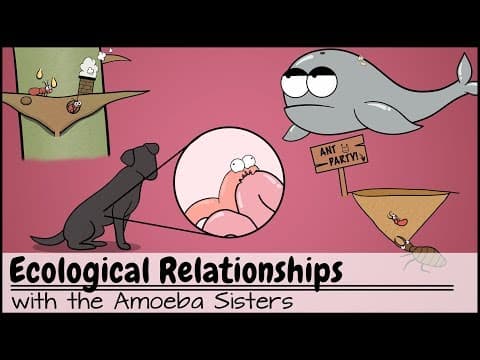
Relationships between members of different species are called interspecific relationships. Each type can be described by its effect on the two species, using + for a benefit, − for harm and 0 for no effect.

Herbivory and predation

In herbivory the consumer usually eats only part of the plant, so the plant survives and regrows; grazed grasses grow from their bases. Predation kills the prey. Both relationships transfer energy and matter from one species to another, and both act as selection pressures: plants evolve thorns and toxins, prey evolve speed and camouflage, and consumers evolve ways of overcoming these defences.

Parasitism and pathogenicity

A parasite benefits by obtaining food and a place to live from its host, and the host is harmed. Parasites are often larger organisms, such as ticks, tapeworms and mistletoe, and many live on their host for a long time. The European mistletoe (Viscum album) grows on the branches of trees such as apple and poplar and takes water and mineral ions from the host's xylem through modified roots.

A pathogen is a microorganism or virus that causes disease. Pathogenicity is therefore a special case in which the harm is disease. Chestnut blight, caused by the fungus Cryphonectria parasitica accidentally introduced from Asia in the early 1900s, spread through the forests of eastern North America and killed almost all mature American chestnut trees (Castanea dentata) within about 50 years.

Mutualism

In mutualism both species benefit. Many mutualisms involve one partner supplying carbon compounds made by photosynthesis and the other supplying something the first cannot get easily on its own, such as nitrogen or mineral ions. Three examples show the range of organisms involved: a plant with bacteria, a plant with a fungus, and an animal with an alga.

Root nodules in the legume family (Fabaceae)

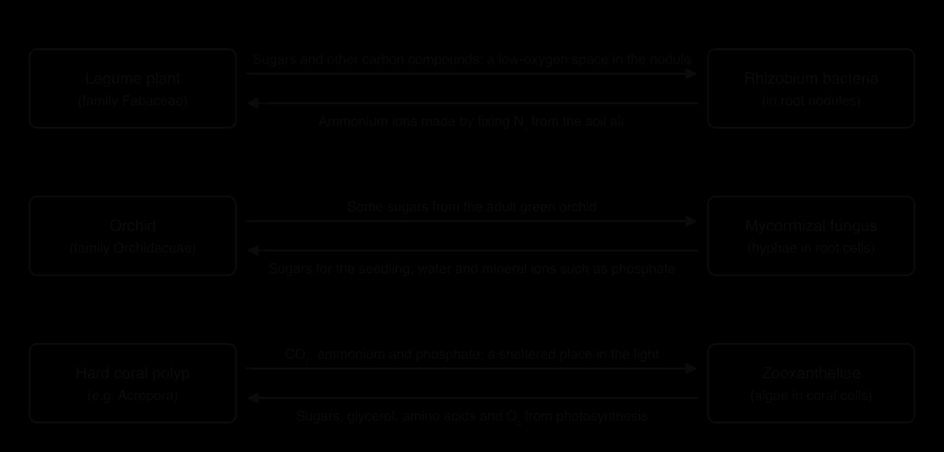
Plants of the legume family, Fabaceae, include peas, beans, clover, lupins and soya. Their roots form root nodules: small swellings containing Rhizobium bacteria. The bacteria live in the soil, enter the root through root hairs, and are enclosed in nodule cells, which become packed with them.

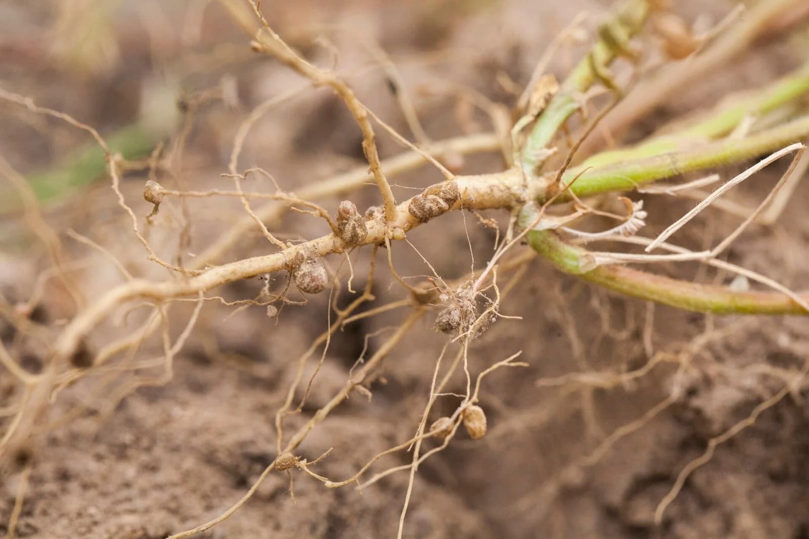
• Benefit to the plant. Nitrogen gas (N₂) makes up about 78% of air, but plants cannot use it. Rhizobium uses the enzyme nitrogenase to fix N₂ from the air spaces in the soil into ammonia, which forms ammonium ions (NH₄⁺). The plant uses the ammonium to make amino acids, proteins and nucleic acids. Legumes can therefore grow well in soils poor in nitrate.

• Benefit to the bacteria. Nitrogen fixation needs a large supply of ATP. The plant supplies the bacteria with sugars and other carbon compounds, made by photosynthesis and carried to the roots in the phloem, which the bacteria use in cell respiration. The nodule also gives the bacteria a protected place to live.

Nitrogenase is inactivated by oxygen, yet the bacteria need oxygen for aerobic respiration. The nodule solves this with leghaemoglobin, an oxygen-binding protein similar to haemoglobin that gives active nodules a pink colour inside. Leghaemoglobin keeps free oxygen at a very low concentration while delivering enough oxygen for respiration. Farmers use this mutualism when they grow clover or beans in rotation with cereals, because the nitrogen fixed by the legumes enriches the soil.

Mycorrhizae in the orchid family (Orchidaceae)

A mycorrhiza is a mutualistic association between a fungus and the roots of a plant. In orchids, the fungal hyphae grow into the cells of the root and form tight coils inside them. The hyphae also spread out through the soil, where they absorb water and mineral ions, and many can digest dead organic matter.

Orchid seeds are as fine as dust and contain almost no food store. A seed in the wild can germinate and grow only if it is infected by a suitable fungus. The fungus supplies the tiny seedling with sugars (obtained from decomposing organic matter in the soil) as well as water and minerals, so for the first months or years the orchid depends entirely on the fungus.

• Benefit to the orchid. Sugars during germination and early growth; water and mineral ions, especially phosphate and nitrogen compounds, throughout life. The network of hyphae has a far larger surface area for absorption than the orchid's own roots.

• Benefit to the fungus. Once the orchid has green leaves and photosynthesises, it passes some of its carbon compounds to the fungus. The orchid root is also a protected habitat for the fungus.

Some orchids, such as the bird's-nest orchid (Neottia nidus-avis), have no chlorophyll and never photosynthesise. They take all their carbon from the fungus throughout life, so the relationship is closer to parasitism of the fungus by the orchid than to mutualism, and only green orchids form a true mutualism with their fungi.

Zooxanthellae in hard corals

Hard corals are the reef-building corals. Each coral is a colony of small animals called polyps, which secrete a skeleton of calcium carbonate. Inside the cells lining the polyp's gut live zooxanthellae: single-celled photosynthetic algae (dinoflagellates), typically millions per square centimetre of coral.

• Benefit to the coral. The zooxanthellae pass most of the sugars, glycerol and amino acids they make by photosynthesis to the coral, which supplies most of its energy needs. They also release oxygen and help the coral deposit its calcium carbonate skeleton faster, which is why coral reefs can grow in clear tropical seas that contain very little food.

• Benefit to the zooxanthellae. The coral provides a protected place in shallow, sunlit water. It also supplies carbon dioxide from its respiration and nitrogen and phosphorus compounds from its waste (such as ammonium), which are scarce in nutrient-poor tropical waters.

The coral and its algae recycle nutrients between them very efficiently, which is why reefs are among the most productive ecosystems on Earth although the surrounding water is poor in nutrients. When the water becomes too warm, the corals expel their zooxanthellae and turn white: coral bleaching. Without the algae the coral starves unless they return, which shows how dependent the coral is on the relationship.

Competition between endemic and invasive species

An endemic species is native to a particular area: it evolved there or arrived without human help. An introduced species has been moved by humans, deliberately or accidentally, to an area outside its natural range. Many introduced species fail to establish, but some spread rapidly and harm the endemic species; these are invasive species.

Introduced species often become invasive because they have a competitive advantage over endemic species in obtaining resources. They may use a resource more efficiently, reproduce faster or tolerate a wider range of conditions. They have also usually left their own predators, parasites and diseases behind, so their populations are not held in check. The endemic species that use the same resources are then restricted to a smaller realised niche, or are lost from the area altogether.

Grey squirrels and red squirrels in Britain

The red squirrel (Sciurus vulgaris) is endemic to Britain. The grey squirrel (Sciurus carolinensis) is native to eastern North America; it was first released in Britain at Henbury Park, Cheshire, in 1876, and further releases followed. Grey squirrels have since spread through most of England and Wales and parts of Scotland, and red squirrels have disappeared from most of the areas they invaded.

The two species eat the same foods: seeds, nuts, buds and fungi. Grey squirrels are larger, spend more time feeding on the ground, live at higher densities and digest acorns more efficiently than red squirrels, which are less able to cope with the tannins acorns contain. In broadleaved woodland, especially oak woodland, greys therefore obtain more energy from the same food supply and outcompete reds. Red squirrels survive mainly in large conifer forests in Scotland and northern England and on islands such as Anglesey and the Isle of Wight, where grey squirrels are absent or do less well.

Grey squirrels also carry squirrelpox virus, which rarely harms them but is usually fatal to red squirrels. Disease is a separate effect from resource competition, and in many areas the two act together. Conservation of red squirrels now combines controlling grey squirrels, managing conifer forests that favour reds, and protecting island populations.

Testing for interspecific competition

Interspecific competition is suspected when two species use the same resource and one does better where the other is absent. Demonstrating competition is difficult, because a species may be rare where another is common for reasons that have nothing to do with competition: the two may simply prefer different soils, temperatures or depths of water. Evidence that one species is more successful in the absence of another therefore indicates competition but does not prove it. Ecologists use three approaches, each with strengths and weaknesses.

Laboratory experiments

In a laboratory experiment the two species are grown separately and together under controlled conditions. In 1934 the Russian ecologist Georgy Gause grew two species of single-celled protist, Paramecium aurelia and Paramecium caudatum, in tubes of culture medium with bacteria as food. Grown separately, each species showed sigmoid growth and reached a stable population. Grown together, P. aurelia continued to thrive but P. caudatum declined until it disappeared from the cultures.

Because temperature, food supply and volume were the same in every tube, the only difference between the single and mixed cultures was the presence of the other species. The decline of P. caudatum can therefore be attributed to competition with P. aurelia for the bacteria, an example of competitive exclusion. The weakness of laboratory experiments is that the conditions are artificial: a simple tube of medium may not reflect what happens in a pond, where the two species can feed in different places.

Field observations by random sampling

In the field, ecologists can record where each species occurs using random quadrats and test whether the two are found together more or less often than expected by chance (using the chi-squared test). Field observations study organisms in natural conditions and can cover large areas and many sites. They show only a correlation, however: if two species rarely occur together, competition is one explanation, but different habitat preferences are another.

Field manipulation by removing one species

In a removal experiment, one species is removed from some plots and left in others (the controls), and the response of the second species is measured. The best-known example is Connell's work on two barnacle species on a Scottish rocky shore, where removing one species allowed the other to survive lower down the shore (studied in detail in B4.2 Ecological niches). Removal experiments combine natural conditions with an experimental test of cause and effect, but they are slow, can be done only with species that are easy to remove, and other factors still vary between plots.

The chi-squared test for association between species

If two species compete, they may be found together less often than expected by chance (a negative association). If they depend on each other, or share the same habitat requirements, they may be found together more often than expected (a positive association). The chi-squared test determines whether the observed pattern differs significantly from what chance alone would produce.

Collecting presence and absence data

Quadrats are placed at random over the study area, often across several sites so that a range of conditions is included. In each quadrat the observer records only whether each species is present or absent. Every quadrat falls into one of four categories: both species present, only species A, only species B, or neither. The four counts are set out in a 2 × 2 contingency table.

Hypotheses

The test begins with two hypotheses. The null hypothesis (H₀) is that there is no association between the two species: their distributions are independent, and any difference between observed and expected frequencies is due to chance. The alternative hypothesis (H₁) is that there is an association between the two species, positive or negative.

Calculating the test statistic

1. Draw the contingency table of observed frequencies (O), with row totals, column totals and the grand total.

2. Calculate the expected frequency (E) for each cell, assuming the null hypothesis: $E = \dfrac{\text{row total} \times \text{column total}}{\text{grand total}}$.

3. For each cell calculate $\dfrac{(O - E)^2}{E}$, then add the four values to give χ².

4. Find the degrees of freedom: (number of rows − 1) × (number of columns − 1). For a 2 × 2 table this is (2 − 1) × (2 − 1) = 1.

5. Compare χ² with the critical value for that number of degrees of freedom at the 5% significance level (p = 0.05).

If χ² is greater than the critical value, the difference between observed and expected frequencies is too large to be explained by chance more than 5% of the time. The null hypothesis is rejected, and the association is statistically significant. If χ² is less than or equal to the critical value, the null hypothesis is accepted (strictly, it cannot be rejected).

Source: standard chi-squared distribution table.

Predator–prey relationships and density-dependent control

Predation is a density-dependent factor. When prey are abundant, predators find food easily, survive well and raise more young, so the predator population grows. More predators then kill more prey, so the prey population falls. With fewer prey, predators starve or fail to breed, and their numbers fall too. With fewer predators, the prey population recovers and the cycle begins again.

Because predators take time to respond, through births and deaths, the predator population lags behind the prey population. Peaks in predator numbers come after peaks in prey numbers, and the two populations oscillate out of step.

Snowshoe hares and Canada lynx

The best-known example comes from the boreal forests of Canada. The Hudson's Bay Company bought furs from trappers for nearly a century, and its records of snowshoe hare and lynx pelts from about 1845 to 1935 show regular cycles in both species with a period of about 10 years. The number of lynx pelts peaked one or two years after the number of hare pelts, as the model predicts. The lynx depends heavily on the hare as its main prey, so lynx numbers follow hare numbers closely.

Field experiments in the Kluane region of the Yukon in the late 1980s and early 1990s tested what drives the hare cycle. In large fenced areas, ecologists added food for the hares, excluded predators, or did both. Adding food or excluding predators alone each raised hare density, but the largest effect came when both were done together. The hare cycle is therefore caused by predation and food supply acting together, which is an example of top-down and bottom-up factors interacting.

Top-down and bottom-up control of populations

Populations in a community can be limited from either end of the food chain. In top-down control, consumers limit the populations of the organisms they eat: predators keep herbivore numbers low, which in turn allows more plants to grow. In bottom-up control, resources limit populations from below: the supply of nutrients and light sets the amount of plant growth, which sets the number of herbivores, which sets the number of predators.

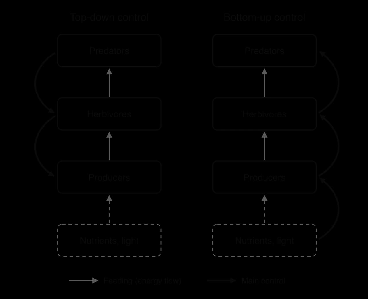
Both types of control operate in every community, but usually one of them is dominant. Which one dominates can change over time or between places.

Top-down control: wolves in Yellowstone

Grey wolves (Canis lupus) were eliminated from Yellowstone National Park in the USA by the 1920s. Without their main predator, elk (Cervus canadensis) became abundant and browsed heavily on young willow and aspen trees, especially along rivers. In 1995 and 1996, 31 wolves captured in Canada were released in the park. Elk numbers on the northern range fell, and elk spent less time feeding in open river valleys where they were easily hunted. Willows and aspen began to recover in some places, and beavers, which depend on willow, became more common.

This chain of effects passing down through several levels is a trophic cascade, and it is a widely cited example of top-down control by an apex predator. The size of the effect is debated: hunting by humans, drought, and predation by bears and cougars also reduced elk numbers, and willow recovery has been patchy. The case shows how difficult it is to separate the causes of change in a real community, where many factors change at once.

Bottom-up control: nutrients and fisheries in upwelling seas

Off the coast of Peru, winds draw cold, nutrient-rich water up from the deep ocean. The nutrients support dense growth of phytoplankton, which feed zooplankton and huge shoals of Peruvian anchoveta (Engraulis ringens), the basis of one of the largest fisheries in the world, and the seabirds and sea lions that eat them. In El Niño years, warm surface water stops the upwelling. With fewer nutrients, phytoplankton production falls and anchoveta numbers crash, along with the seabirds that depend on them. The community is controlled mainly from the bottom up: the supply of nutrients limits every level above it.

Allelopathy and antibiotics: chemical competition

Some organisms compete by releasing chemical substances into the environment that harm or kill potential competitors. In plants this is called allelopathy; in microorganisms the chemicals are often antibiotics. In both cases the chemical reduces competition for resources such as light, water, space and nutrients.

Allelopathy: black walnut

The black walnut tree (Juglans nigra) of eastern North America produces juglone, a compound that is released from its roots, fallen leaves and nut husks into the soil. Juglone inhibits respiration and growth in many other plants, including tomatoes, potatoes, apple trees and many garden shrubs, which wilt and die near the tree. Black walnut therefore suffers less competition for water, minerals and light within the area its roots reach.

Secretion of antibiotics: Penicillium

Fungi and bacteria in soil and on decaying matter compete intensely for nutrients. Many secrete antibiotics that kill or stop the growth of competing bacteria. The mould Penicillium secretes penicillin, which prevents bacteria from building their cell walls. Penicillin was discovered in 1928 when Alexander Fleming noticed that bacterial colonies did not grow around a Penicillium colony that had contaminated a culture plate. Soil bacteria of the genus Streptomyces produce many more antibiotics, including streptomycin. Medicine uses these chemicals, but their original function in nature is competition between microorganisms.

Exam practice

Questions on populations and communities appear in Paper 1A as multiple-choice items on sampling, growth curves and types of relationship, and in Paper 1B as data-based questions on quadrat data, the Lincoln index and the chi-squared test. Paper 2 uses data on real populations (growth curves, predator–prey cycles, invasive species) and extended responses asking you to explain density-dependent control, describe mutualism or evaluate methods of testing for competition. Common command terms are calculate, explain, outline, suggest and evaluate.

Extended-response questions on populations and communities reward structured answers: a definition, the mechanism in steps, and a named example. For mutualism, give the benefit to each partner in every example. For tests of competition, compare an experiment and an observation explicitly, and say what each can and cannot show.

Self-check

• To do:

  I can define a population and explain how reproductive isolation separates populations of one species.

• To do:

  I can explain why population size is estimated by random sampling and what sampling error is.

• To do:

  I can describe random quadrat sampling, calculate a mean and standard deviation, and estimate population size.

• To do:

  I can use the Lincoln index and state and explain its assumptions.

• To do:

  I can define carrying capacity and explain how density-dependent factors control population size by negative feedback.

• To do:

  I can sketch and annotate exponential and sigmoid growth curves and test for exponential growth on a log scale.

• To do:

  I can describe how to model population growth with yeast or duckweed and compare observed and expected curves.

• To do:

  I can give real examples of intraspecific competition and cooperation in plants and animals.

• To do:

  I can describe the six interspecific relationships with an example of each, and explain the benefits to both partners in three mutualisms.

• To do:

  I can explain how an invasive species outcompetes an endemic species, using a named example.

• To do:

  I can evaluate laboratory experiments, field observations and removal experiments as tests for competition, and carry out a chi-squared test for association.

• To do:

  I can explain predator–prey cycles, top-down and bottom-up control, allelopathy and antibiotic secretion with named examples.

[4 max]