4.9 The normal distribution

Many quantities measured on a continuous scale cluster around a central value, with values further from the centre becoming steadily rarer: the heights of adults, the masses of loaves from a bakery, the birth weights of babies, the errors made when measuring the same length many times. Plotted as a histogram, data of this kind form a symmetric, bell-shaped pattern. The normal distribution is the probability model for this pattern.

The normal distribution is the most important distribution in statistics. It is a model for continuous measurements rather than for counts, it is described completely by just two numbers, the mean and the standard deviation, and its probabilities are found as areas under a curve.

Continuous random variables

From a histogram to a curve

A discrete random variable, such as the number of heads in 10 coin tosses, takes separate values, and each value has its own probability (4.7). A measurement such as a mass or a time can take any value in an interval, so it is modelled by a continuous random variable. There are infinitely many possible values, and listing a probability for each is impossible.

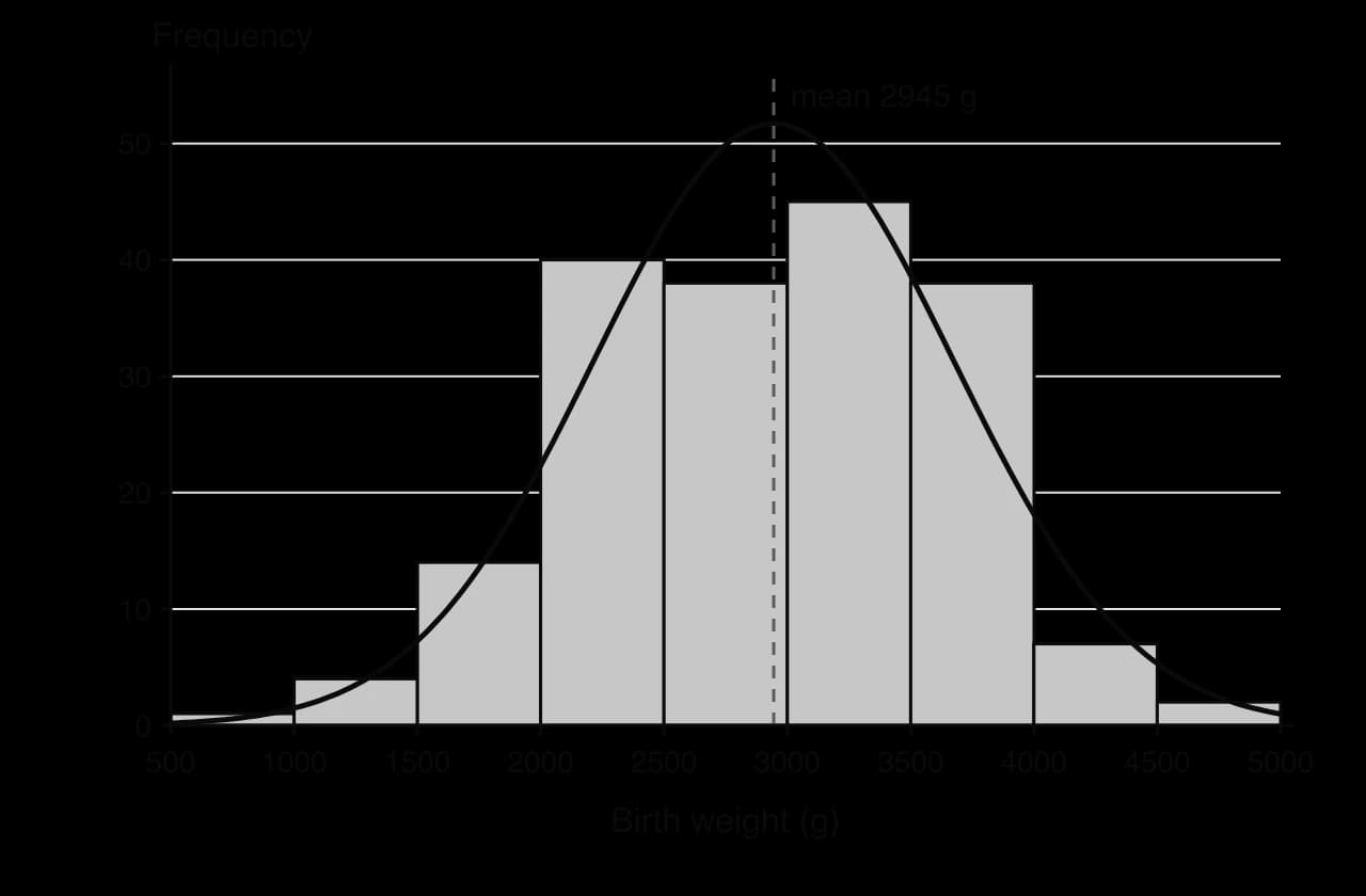
The way forward comes from a histogram. The histogram of the birth weights of 189 babies, drawn with classes of 500 g, rises to a peak near the mean of about 2945 g and falls away on both sides. With more data and narrower classes, the tops of the bars would follow a smooth curve more and more closely. That smooth curve is the probability model for the data.

Probability as area

For a continuous random variable, probabilities are areas under the curve. The curve is drawn so that the total area under it is $1$, and the probability that $X$ lies between $a$ and $b$ is the area under the curve between $x = a$ and $x = b$. In a histogram drawn with relative frequencies, the area of each bar is the proportion of the data in that class, so the idea is the same one, made smooth.

A single value has no width, so the area above it is zero. For a continuous random variable,

This sounds strange at first, but it matches measurement in practice. The probability that a baby weighs exactly 3000.000… g is zero; the probability that a baby weighs between 2950 g and 3050 g is not. One useful consequence is that strict and non-strict inequalities give the same probability:

The normal distribution

Definition and notation

A normal distribution is fixed by two numbers: its mean $\mu$, which sets the centre, and its standard deviation $\sigma$, which sets the spread. The notation records the mean and the variance $\sigma^2$.

The second number in the brackets is the variance, not the standard deviation. A variable described as $X \sim N(50, 16)$ has standard deviation $\sigma = \sqrt{16} = 4$. To avoid confusion, many questions write the variance as a square, $N(50, 4^2)$.

The shape of the normal curve

The heights of adult women in a particular country are modelled by $X \sim N(163, 6.5^2)$, in centimetres. The graph of the model is the normal curve with $\mu = 163$ and $\sigma = 6.5$.

Every normal curve has the same set of properties.

• Symmetric about the mean. The curve is the same on both sides of the line $x = \mu$, so $P(X < \mu) = P(X > \mu) = 0.5$.

• Bell-shaped, with one peak. The single peak is at $x = \mu$, and the curve falls away steadily on both sides.

• Mean = median = mode. The symmetry puts the median at the centre, and the peak puts the mode there as well, so all three equal $\mu$.

• Total area 1. The whole area under the curve represents the probability of all possible values.

• Never touches the axis. The curve approaches the horizontal axis as $x \to \pm\infty$, so in theory any value is possible. In practice values further than about $3\sigma$ from the mean are very rare.

• Points of inflexion at $\mu \pm \sigma$. The curve changes from bending downwards to bending upwards one standard deviation either side of the mean, which shows where $\sigma$ is on a sketch.

The curve has an equation, given here for reference:

The area under this curve cannot be found with the integration methods of the course, which is why normal probabilities come from a GDC or, by hand, from a few remembered values.

The effect of the mean and the standard deviation

Changing $\mu$ slides the curve left or right without changing its shape: it is a horizontal translation. Changing $\sigma$ changes the spread. A larger standard deviation stretches the curve horizontally, and because the total area must stay equal to $1$, the curve also becomes lower. A smaller standard deviation gives a taller, narrower curve. The height of the peak is $\frac{1}{\sigma\sqrt{2\pi}}$, so doubling $\sigma$ halves the height of the peak.

The 68–95–99.7 rule

The three key percentages

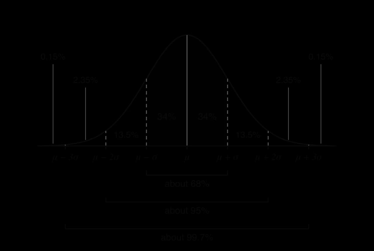
All normal curves have the same shape once they are scaled by their own mean and standard deviation. As a result, the proportion of values within one, two or three standard deviations of the mean is the same for every normal distribution. These three proportions form the 68–95–99.7 rule.

More precise values are 68.27%, 95.45% and 99.73%. Splitting each band in half by symmetry, and taking differences between the bands, gives the percentage in every strip one standard deviation wide.

The strip percentages come from simple arithmetic on the rule:

Using the rule

IQ scores are designed so that, in the population used to set the scale, they have a mean of 100 and a standard deviation of 15. They are modelled by $X \sim N(100, 15^2)$, which makes them a natural first example of the rule.

The rule also works backwards. If a range is known to hold about 95% of the values, it must stretch two standard deviations either side of the mean, and both parameters can be read off.

Drawing the region for a probability

Sketch first, then calculate

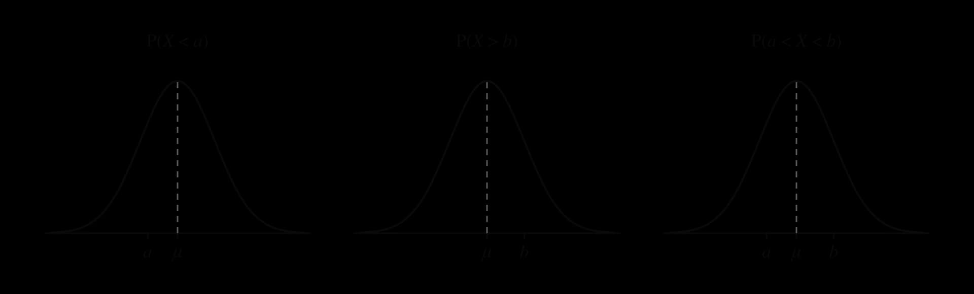
Every normal probability is an area, and the quickest way to see which area is needed is a sketch. Draw a symmetric bell, mark the mean in the middle, mark the boundary values in the right places (left of the mean if smaller, right of it if larger), and shade the region the question asks for. The three basic shapes are a left tail, a right tail and a region between two values.

A sketch also checks the size of an answer. If the shaded region is a small tail, the probability must be small; if it covers more than half the curve, the probability must be greater than $0.5$. An answer that disagrees with its sketch signals an error, such as a wrong inequality or a wrong value of $\sigma$.

Symmetry without a calculator

The symmetry of the curve gives exact relations between areas. Values equally far from the mean on opposite sides cut off equal tails:

and each half of the curve has area $0.5$. These two facts often give a probability from one piece of information, with no calculator at all.

Normal probabilities with a GDC

The normal cdf function

A graphic display calculator (GDC) finds normal areas with its normal cdf function (cdf stands for cumulative distribution function). It needs four inputs: the lower boundary, the upper boundary, the mean $\mu$ and the standard deviation $\sigma$. For a tail with no second boundary, enter a very large number in its place, such as $-10^{99}$ for "no lower boundary" or $10^{99}$ for "no upper boundary". Any number more than about ten standard deviations from the mean gives the same answer to many decimal places.

Because $P(X = a) = 0$, "at most" and "less than" give the same probability, and so do "at least" and "more than". A probability found this way can be checked against the rule: a boundary one standard deviation above the mean, for example, should give a right tail close to $0.16$.

Spread versus centre

Two normal distributions can be compared through their probabilities as well as their parameters. A small change in the standard deviation often matters more than a change in the mean, especially for probabilities in the tails.

Conditional probabilities

A conditional probability with a normal variable uses the formula for conditional probability from 4.11, $P(A \mid B) = \frac{P(A \cap B)}{P(B)}$, with each event written as an inequality. The intersection of two one-sided inequalities in the same direction is simply the stricter one.

Inverse normal calculations

Finding a boundary from a probability

A normal probability calculation starts with a boundary and finds an area. An inverse normal calculation runs the other way: it starts with an area and finds the boundary. Questions of this kind ask for a value such as the height exceeded by only 5% of people, the mass below which 10% of products fall, or the score needed to be in the top 2%.

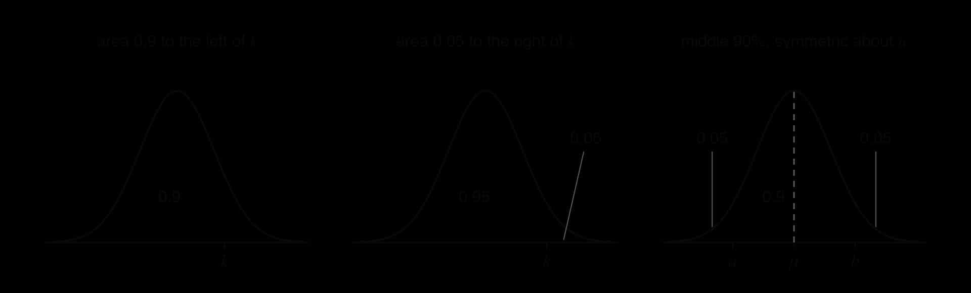
The inverse normal function of a GDC takes the area to the left of the boundary, together with $\mu$ and $\sigma$, and returns $k$. Some calculators also accept a right-tail or a central area; when only the left area is accepted, every other case must first be rewritten as an area to the left.

The three cases in the figure cover almost every inverse normal question:

1. Area to the left given, $P(X < k) = p$: enter $p$ directly.

2. Area to the right given, $P(X > k) = p$: enter $1 - p$, the area to the left.

3. Central area given, $P(a < X < b) = p$ with $a$ and $b$ symmetric about $\mu$: each tail holds $\frac{1 - p}{2}$

Inverse normal problems in context

In context, the answer to an inverse normal question often has to be interpreted: rounded in the right direction for whole-number scores, or compared with a practical limit. Decide what the boundary means before rounding it.

When a normal model is suitable

Where normal distributions come from

A quantity tends to be approximately normal when it is the combined result of many small, independent effects, none of which dominates. An adult's height depends on many genes and on many influences such as diet and health, each adding or subtracting a little. Repeated measurements of one length differ through many small disturbances in the instrument, the reading and the conditions, which is why measurement errors are often close to normal. The same reasoning applies to birth weights of babies born at full term, the masses of products from a machine, and the scores on a long test made of many questions.

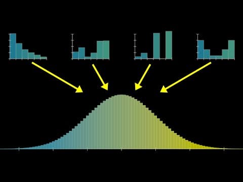
The video shows a Galton board, in which balls bounce left or right off many pins and pile up in a bell shape, and then explains why sums of many random effects approach a normal curve.

Checking real data against a normal model

A normal model is a simplification, and real data are never exactly normal. A model is reasonable when the data show the main features of the normal curve. Four checks are useful:

1. Shape. A histogram of the data is roughly symmetric, with a single peak in the middle.

2. Centre. The mean, median and mode are close to each other.

3. Spread. About 68% of the data lie within one standard deviation of the mean, and about 95% within two.

4. Range. The interval from $\mu - 3\sigma$ to $\mu + 3\sigma$ contains no impossible values, such as negative lengths or times.

The birth weights of the 189 babies pass all four checks. The histogram is close to symmetric with one peak, the mean (2945 g) and median (2977 g) are close, and the proportions of the data within one, two and three standard deviations of the mean are 67.7%, 96.3% and 99.5%, very close to 68%, 95% and 99.7%.

When the normal model fails

Several kinds of data are clearly not normal, and a normal model gives misleading probabilities for them.

• Skewed data. Incomes, house prices, waiting times and the lengths of rivers have a long tail on one side. The mean is pulled towards the tail and differs noticeably from the median.

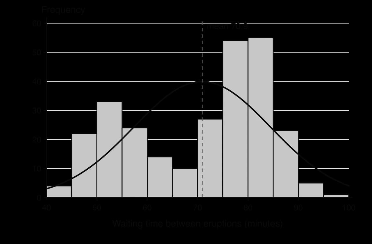
• Bimodal data. Data with two peaks, such as the waiting times between eruptions of the Old Faithful geyser, come from two different groups mixed together.

• Data near a natural limit. If a quantity cannot be negative and its mean is less than about three standard deviations above zero, a normal model gives a noticeable probability to impossible negative values.

• Discrete data with few values. Counts such as the number of children in a family take only a handful of values; a binomial or other discrete model is more suitable.

Exam-style questions on the normal distribution

Normal distribution questions on calculator papers test the setting up (the distribution, a sketch, the probability statement) as much as the GDC work. On non-calculator papers they rely on symmetry and the 68–95–99.7 rule. Questions often end by combining a normal probability with the binomial distribution (4.8) or with conditional probability.

The second question needs no calculator. Every value in it is placed symmetrically about the mean, so symmetry and the total area of 1 give each answer.

Self-check

• To do:

  I can describe the properties of the normal curve: symmetric, bell-shaped, mean = median = mode, total area 1.

• To do:

  I can explain the effect of changing $\mu$ or $\sigma$ on the normal curve.

• To do:

  I can tell whether a number in $N(\mu, \sigma^2)$ is the variance or the standard deviation, and enter $\sigma$ into a GDC.

• To do:

  I can use the 68–95–99.7 rule, forwards and backwards, without a calculator.

• To do:

  I can sketch a normal curve and shade the region for a probability.

• To do:

  I can find $P(X < a)$, $P(X > b)$ and $P(a < X < b)$

• To do:

  I can find a boundary from a given left-tail, right-tail or central probability.

• To do:

  I can decide whether a normal model suits a real situation and give a reason.

• A ~ N(150, 10²)
• B ~ N(160, 20²)

(b) Orchard B's apples are heavier on average, since $160 > 150$. They also vary more, since their standard deviation is $20$ g compared with $10$ g.

(c) The height of a peak is $\frac{1}{\sigma\sqrt{2\pi}}$, so the ratio of the heights is

Curve A's peak is twice as high as curve B's.

(c) The region from 42 to 58 is split equally by the mean:

(d) Everything except the right tail:

(b) A score must be above $130.80\ldots$ to be in the top 2%, so the lowest qualifying whole-number score is 131. Rounding down to 130 would admit more than 2% of people.

[2]2 marks