4.8 The binomial distribution

Many random processes repeat the same simple trial a fixed number of times and count how often something happens: the number of free throws a basketball player scores out of 10, the number of faulty items in a box of 50, the number of correct answers when a student guesses on a multiple-choice test. When the trials are independent and each has the same probability of success, the count follows the binomial distribution. It is the most widely used discrete probability distribution.

The binomial distribution has a formula for every probability, a simple expression for its mean and variance, and built-in functions on every graphic display calculator (GDC). It connects the counting methods of the binomial theorem (1.9) with the expected values of discrete random variables (4.7).

When the binomial model applies

Bernoulli trials

The building block of the binomial distribution is a single trial with exactly two outcomes. The outcome being counted is called a success and the other a failure, whatever they mean in context: a "success" may be a faulty item or a patient who catches a disease.

Many trials with more than two outcomes can be turned into Bernoulli trials by grouping the outcomes. Rolling a die has six outcomes, but "roll a six" and "do not roll a six" are two, with $p = \frac{1}{6}$.

The four conditions

A random variable $X$ follows a binomial distribution when it counts the number of successes in a sequence of Bernoulli trials that satisfy four conditions.

1. Fixed number of trials: the number of trials $n$ is decided in advance.

2. Two outcomes: each trial results in success or failure.

3. Constant probability: the probability of success $p$ is the same for every trial.

4. Independence: the outcome of one trial does not affect the outcome of any other.

The conditions are assumptions about the real situation, and in context they are often only approximately true. A basketball player's free throws are usually modelled as independent with a constant success rate, although tiredness or confidence may change the rate during a game. Stating which assumptions a model makes, and judging whether they are reasonable, is part of modelling with the binomial distribution.

The binomial probability formula

Deriving the formula from a tree diagram

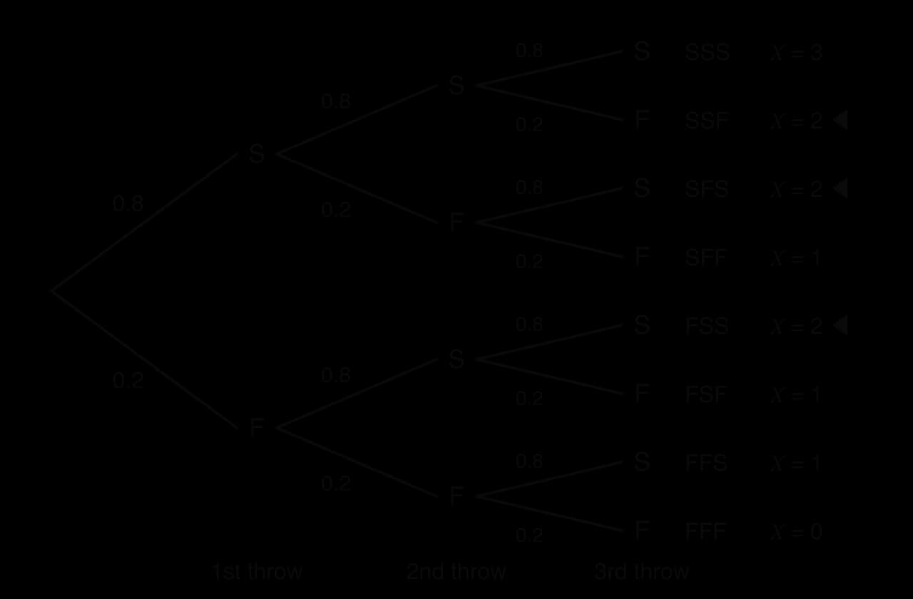
A basketball player scores each free throw with probability $0.8$, independently of the others. She takes three free throws. Let $X$ be the number she scores. Each throw is a success S or a failure F, so there are $2^3 = 8$ possible sequences.

Three sequences give exactly two successes: SSF, SFS and FSS. Each contains two factors of $0.8$ and one of $0.2$, so each has probability $0.8^2 \times 0.2 = 0.128$, and

The same reasoning applies to any number of successes. With $n$ trials, a sequence with $r$ successes and $n - r$ failures has probability $p^r(1 - p)^{n - r}$, whatever the order. The number of such sequences is the number of ways to choose which $r$ of the $n$ trials are the successes, the binomial coefficient $\binom{n}{r}$ from 1.9. Here $\binom{3}{2} = 3$.

Applying the formula to each value of $r$ gives the complete distribution of the number of free throws scored, $X \sim B(3, 0.8)$.

Why the probabilities add up to 1

The terms $\binom{n}{r}p^r(1 - p)^{n - r}$ are exactly the terms of the binomial expansion of $\left(p + (1 - p)\right)^n$, which is where the distribution gets its name. Their sum is therefore

so every binomial distribution is a valid probability distribution. For $B(3, 0.8)$: $0.008 + 0.096 + 0.384 + 0.512 = 1$.

Using the formula

To use the formula, identify $n$, $p$ and the number of successes $r$, then substitute. Exact answers come from fractions when $p$ is a simple fraction; otherwise give answers to 3 significant figures.

When $p$ is a simple fraction, the formula gives exact answers that can be worked out by hand. Complements are especially useful: "at least one success" is the complement of "no successes", and $P(X = 0) = (1 - p)^n$ is a single power.

The shape of a binomial distribution

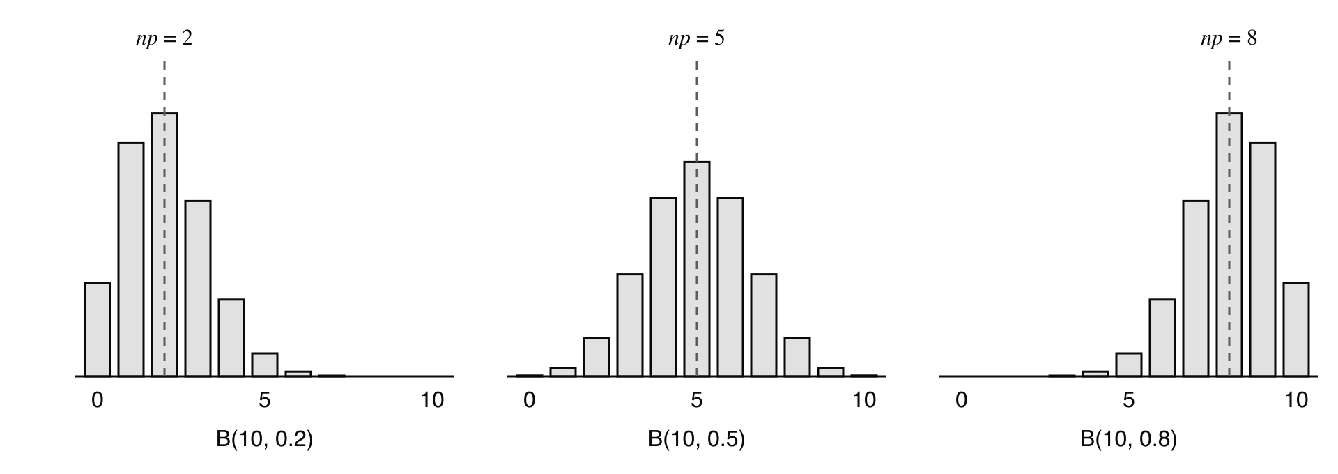
The shape of $B(n, p)$ depends on $p$. When $p = 0.5$ the distribution is symmetric about $\frac{n}{2}$, because successes and failures are equally likely. When $p$ is small, most of the probability sits on small values and the distribution has a long tail to the right (positive skew). When $p$ is large, the picture is reflected and the tail is to the left.

The reflection in the figure is a general fact. If $X \sim B(n, p)$ counts successes, then $n - X$ counts failures, and $n - X \sim B(n, 1 - p)$. For example, the probability of exactly 2 successes in $B(10, 0.2)$ equals the probability of exactly 8 successes in $B(10, 0.8)$.

Cumulative probabilities and the GDC

The binomial pdf and cdf functions

Questions often ask for the probability of a range of values, such as "at most 3" or "at least 5". Adding many terms of the formula by hand is slow, so a GDC is normally used. It has two binomial functions:

• the binomial pdf gives a single probability, $P(X = r)$;

• the binomial cdf gives a cumulative probability, $P(X \le r)$, the sum $P(X = 0) + P(X = 1) + \dots + P(X = r)$.

Some calculators ask for a lower and an upper bound in the cdf, and then give $P(a \le X \le b)$ directly. Others give only $P(X \le r)$, and every other range must be rewritten in that form, using the complement and the fact that $X$ takes only whole-number values.

Translating words into inequalities

Because $X$ takes only the values $0, 1, 2, \dots, n$, the inequality $X > 3$ means the same as $X \ge 4$, and $X < 3$ means $X \le 2$. Each phrase in a question becomes an inequality, then a calculation with the cdf.

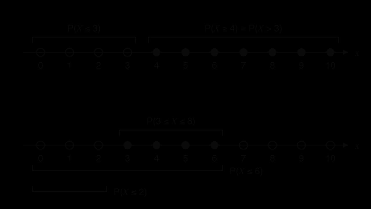
A number line of the whole numbers $0, 1, 2, \dots$ makes the end points clear. Mark the values that are included, then see which cumulative probability covers them.

The guessing student in a 10-question multiple-choice test gives a second example with the cdf. The probability of passing with 5 or more correct answers by guessing alone is

for $X \sim B(10, 0.25)$, so fewer than 1 in 12 students who guess everything would pass.

Mean and variance of the binomial distribution

The mean np

If a player scores 80% of her free throws, then in 40 attempts she is expected to score about $40 \times 0.8 = 32$. In general, each of the $n$ trials succeeds with probability $p$, so the long-run mean number of successes is $np$. This is the expected number of occurrences from 4.5, and it is the expected value $E(X)$ of the binomial random variable.

For a small case, the result can be checked with $E(X) = \sum x\,P(X = x)$ from 4.7. For $X \sim B(3, 0.8)$,

The variance np(1 − p)

The variance of a random variable measures how spread out its values are about the mean, in the same way that the variance of a data set does (4.3). For the binomial distribution it has a simple formula, and the standard deviation is its square root.

The variance $np(1 - p)$ is largest when $p = 0.5$ and becomes small when $p$ is close to 0 or 1. This matches intuition: if success is almost certain, the number of successes is almost certain too, and there is little spread. A larger number of trials gives a larger variance, but the proportion of successes, $\frac{X}{n}$, becomes less spread out as $n$ grows, which is the informal law of large numbers from 4.5.

Since $np$ and $np(1 - p)$ are two equations in $n$ and $p$, a given mean and variance determine the distribution. Dividing the variance by the mean removes $n$ and leaves $1 - p$.

Finding n or p

Finding the number of trials n

A common practical question asks how many trials are needed to make an event likely enough: how many components to test, how many people to survey, how many attempts to make. When the event is "at least one success", the complement $P(X = 0) = (1 - p)^n$ turns the problem into an exponential inequality, which logarithms solve.

For events such as "at least two successes", there is no simple algebraic route. A GDC table of values solves the problem: enter the probability as a function of $n$, for example $1 - P(X \le 1)$ with the binomial cdf, and scroll through values of $n$ until the probability first passes the target.

Finding the probability of success p

When $p$ is unknown, a given probability gives an equation in $p$. If the event is $X = 0$ or $X = n$, the equation is a single power and can be solved exactly. If it is a single value of $r$ such as $P(X = 1) = P(X = 2)$, the common factors cancel and the equation simplifies.

For a cumulative probability, the equation in $p$ is a polynomial that generally cannot be solved by hand, so a GDC is used: either graph $y = P(X \le r)$ as a function of $p$ and find its intersection with the target value, or use the equation solver.

Combining the binomial distribution with other probability

Binomial distributions in two stages

The probability of success in one binomial model is sometimes itself a binomial probability. For example, a "good day" might be defined by the number of successes during the day, and then the number of good days in a week is a second binomial count. Work out the first probability fully, keep it unrounded, and use it as $p$ in the second distribution.

Conditional probability with a binomial variable

Conditional probabilities use the formula $P(A \mid B) = \frac{P(A \cap B)}{P(B)}$ from 4.6, with the events written as inequalities in $X$. Find the intersection of the two inequalities first.

Exam-style questions on the binomial distribution

Binomial questions appear on both calculator and non-calculator papers. With a GDC, the work is mostly in identifying the distribution and translating the words into inequalities; without one, the formula and complements must be used by hand.

Self-check

• To do:

  I can state the four conditions for a binomial model and decide whether a situation meets them.

• To do:

  I can explain why $P(X = r) = \binom{n}{r}p^r(1 - p)^{n - r}$, using a tree diagram.

• To do:

  I can calculate binomial probabilities by hand, including with complements such as $1 - (1 - p)^n$.

• To do:

  I can translate "at most", "at least", "more than", "fewer than" and "between" into inequalities and use the binomial cdf.

• To do:

  I can find and interpret the mean $np$, the variance $np(1 - p)$ and the standard deviation.

• To do:

  I can find $n$ and $p$ from a given mean and variance.

• To do:

  I can find the least $n$ for a probability to exceed a target, using logarithms or a GDC table.

• To do:

  I can find an unknown $p$ from a given probability, by algebra or with a GDC.

• To do:

  I can solve two-stage and conditional problems involving a binomial distribution.

$= 1228.8$, so approximately $1230$ households A1

Note: Accept $1229$ or $1228.8$.

(b) No. The number of trials is not fixed in advance: $X$ counts trials, not successes.

(c) No. Without replacement, the probability of a heart changes from card to card (it is $\frac{13}{52}$ for the first card, but $\frac{12}{51}$ for the second if the first was a heart), so the trials are not independent and $p$ is not constant.

(d) Yes, assuming the guesses are independent and each is correct with probability $\frac{1}{4}$: $X \sim B(20, 0.25)$.

(e) No. Each roll has six outcomes and $X$ is a total of scores, not a count of successes.

(b) Use the complement of "no successes":

Since $0 < p < 1$, both $p$ and $(1 - p)^3$ are non-zero, so you can divide by $5p(1 - p)^3$:

(b) Use the formula with $r = 1$:

(c) $E(X) = 3 \times 0.4 = 1.2$ and $\operatorname{Var}(X) = 3 \times 0.4 \times 0.6 = 0.72$.