4.14 Continuous random variables

The expected value of a discrete random variable (4.7) describes where its distribution is centred, but two random variables with the same mean can behave very differently. A game that pays $\$1$ every time and a game that pays $\$100$ once in a hundred plays both have an expected prize of $\$1$, yet the second is far riskier. The variance of a random variable measures this difference in spread.

Many quantities are not counted but measured: the time a customer waits, the lifetime of a component, the mass of a bag of flour. These are continuous random variables, which can take any value in an interval. Their probabilities are described by a curve, the probability density function, and found as areas under it by integration. The same ideas of mean, median, mode and variance then apply, with sums replaced by integrals.

Variance of a discrete random variable

Measuring the spread of a random variable

For a set of data, the variance is the mean of the squared deviations from the mean (4.3). A random variable has a variance defined in the same way, with probabilities in place of relative frequencies. Squaring the deviations makes every term positive, so that values above and below the mean do not cancel, and gives more weight to values far from the mean.

For the two games, let $A$ be the prize in the first and $B$ the prize in the second. $A = 1$ with certainty, so every deviation is 0 and $\operatorname{Var}(A) = 0$. $B$

The computational form

Subtracting $\mu$ from every value is slow and leads to awkward decimals. Expanding the bracket gives a quicker formula. Using $\sum x\,P(X = x) = \mu$ and $\sum P(X = x) = 1$

Here $E(X^2) = \sum x^2\,P(X = x)$ is the expected value of $X^2$

Variance is measured in squared units (dollars squared, for example), which are hard to interpret. Taking the square root returns to the units of $X$.

Continuous random variables

From counting to measuring

A discrete random variable takes separate values, each with a positive probability. A measured quantity such as a waiting time can take any value in an interval, and there are infinitely many values in any interval, so they cannot each have a positive probability. The probability that a bus arrives after exactly $4.000\ldots$ minutes, to infinitely many decimal places, is 0. Probabilities are given instead to intervals of values, such as "between 4 and 5 minutes".

A histogram of many measured waiting times, drawn with relative frequency density on the vertical axis, has total area 1. As more data are collected and the class widths shrink, the tops of the bars approach a smooth curve. That curve is the model for the random variable, and the area under it over an interval is the probability that $X$ falls in that interval.

Probability density functions

In practice $f$ is non-zero only on a finite interval, called its domain, and $f(x) = 0$ everywhere else. The infinite integral then becomes an ordinary definite integral over the domain. The two conditions match those for a discrete distribution: probabilities are never negative, and the total probability is 1.

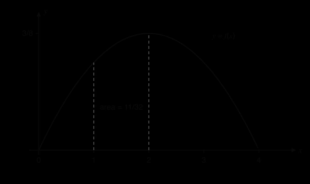
The value $f(x)$ is a probability density, not a probability. It can be greater than 1, as long as the total area is 1: the pdf $f(x) = 3x^2$ for $0 \le x \le 1$

Checking whether a function is a valid pdf

Both conditions must be checked. A function whose integral over its domain is 1 can still fail to be a pdf if it takes negative values.

The continuous uniform distribution

The simplest pdf is constant on an interval. If buses leave a stop exactly every 10 minutes and a passenger arrives at a random time, every waiting time from 0 to 10 minutes is equally likely, and the pdf is a horizontal line.

The area under a uniform pdf is a rectangle, so probabilities can be found without integrating. For the bus, the probability of waiting more than 7 minutes is $(10 - 7) \times \frac{1}{10} = 0.3$.

Piecewise probability density functions

A pdf can be defined by different formulas on different parts of its domain. To find a probability over an interval that crosses a boundary between pieces, split the integral at the boundary and add the parts. The condition that the total area is 1 then involves every piece.

Mode and median of a continuous random variable

The mode

The mode of a data set is its most common value. For a continuous random variable, the corresponding idea is the value where the probability is most densely packed, the highest point of the pdf.

The maximum of $f$ is found with the methods of calculus. It may be a stationary point, where $f'(x) = 0$ and $f''(x) < 0$

The median

The median splits a data set into two halves. For a continuous random variable, it splits the area under the pdf into two halves, each of area $0.5$.

To find $m$, integrate $f$ from the lower end of the domain to $m$, set the result equal to $0.5$ and solve for $m$. The equation is often a quadratic or a polynomial of higher degree. Only a solution inside the domain can be the median; the others must be rejected. When the equation cannot be solved by hand, a GDC solver or graph gives $m$.

For a piecewise pdf, first decide which piece contains the median by finding the area of the first piece. In the help-desk example, the area from 0 to 2 is $\frac{1}{2} \times 2 \times \frac{1}{3} = \frac{1}{3} < 0.5$

Mean, variance and standard deviation

Expected value of a continuous random variable

For a discrete random variable, $E(X) = \sum x\,P(X = x)$ weights each value by its probability. For a continuous random variable, the probability that $X$ lies in a narrow interval of width $\delta x$ near $x$

The second form of the variance is the continuous version of $E(X^2) - [E(X)]^2$, with $E(X^2) = \int x^2 f(x)\,dx$

When the pdf is symmetric about a line $x = c$, the mean (and the median) is $c$, with no integration needed. The pdf $\frac{3}{32}x(4 - x)$

Mean, median and mode together

For the component lifetime pdf $f(x) = \frac{12}{625}x^2(5 - x)$, the three measures of centre are all different, and their order shows the shape of the distribution. The mode was found by differentiation. The mean and the median need integration.

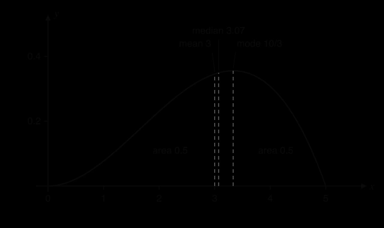
The order mean $<$ median $<$ mode is typical of a distribution with a long tail to the left (negative skew). The pdf $\frac{2}{25}(5 - x)$ has its long tail to the right, and the order is reversed: mode $0 <$

The variance of the uniform waiting time

The variance of a uniform distribution grows with the length of its interval, as the spread of equally likely values grows.

Linear transformations of a random variable

The rules for aX + b

A random variable is often converted to new units or to a new quantity by a linear formula: a temperature in degrees Celsius to degrees Fahrenheit, a score to a prize of $\$3$ per point minus a $\$5$ stake. The new random variable $aX + b$ has a mean and variance that follow directly from those of $X$.

The rule for the mean follows from the definition. For a discrete random variable,

and the continuous case is the same with integrals. For the variance, every deviation from the mean is multiplied by $a$, because $(ax + b) - (a\mu + b) = a(x - \mu)$. Squaring multiplies each squared deviation by $a^2$

Adding $b$ moves the whole distribution along by $b$ without changing its spread, so $b$ does not appear in the variance.

Exam-style questions on continuous random variables

Questions on probability density functions bring together integration, solving equations and the properties of distributions. Non-calculator questions use pdfs that integrate exactly; calculator questions often use piecewise pdfs and ask for a median or variance that needs a GDC.

Self-check

• To do:

  I can calculate $\operatorname{Var}(X) = E(X^2) - [E(X)]^2$ and the standard deviation for a discrete random variable.

• To do:

  I can explain why $P(X = a) = 0$