5.1 Limits and the derivative

Calculus is the mathematics of change. Many quantities change at a rate that is itself changing: a falling stone speeds up, the level of carbon dioxide in the atmosphere rises faster each decade, and the number of people using a new app grows quickly and then levels off. A straight line has one gradient everywhere, but a curve is steeper in some places than in others. Differential calculus answers the question "how steep is the curve at this exact point?", or, in a context, "how fast is this quantity changing at this exact moment?"

The answer rests on the idea of a limit: the value that a quantity approaches as something else gets closer and closer to a fixed value. Using limits, the gradient of a curve at a point is defined as the value that the gradients of nearby chords approach. The result is the derivative, the central object of the rest of Topic 5.

Rates of change

Measuring how fast a quantity changes

A rate of change compares how much one quantity changes with how much another quantity changes at the same time. Speed is the most familiar example: a car that travels $150$ km in $2$ hours has an average speed of $75$ km per hour. Many other rates appear in science, economics and daily life, such as litres per minute for water flowing into a tank, dollars per item for the cost of producing goods, and degrees Celsius per hour for a cooling drink.

When $y$ is plotted against $x$, a rate of change is a gradient. For a straight line the rate is constant, because the gradient is the same everywhere. For a curve the rate changes from point to point, which is why a new tool is needed.

The average rate of change

Over an interval from $x = a$ to $x = b$, the change in the function is $f(b) - f(a)$ and the change in the input is $b - a$. Dividing one by the other gives the average rate of change over the interval.

A chord of a curve is a straight line segment joining two points on it. The average rate of change describes the overall change between the two points, but it hides what happens in between: a car with an average speed of $75$ km per hour may have stopped at traffic lights and then driven at $100$ km per hour.

The table gives the annual mean concentration of carbon dioxide in the atmosphere, measured at the Mauna Loa Observatory in Hawaii, in parts per million (ppm). (Data: NOAA Global Monitoring Laboratory, Mauna Loa annual mean CO₂, 2025 release.)

The idea of a limit

Approaching a value

Consider the function

Substituting $x = 2$ gives $\frac{0}{0}$, which has no value, so $f(2)$ is not defined. The function is defined for every other value of $x$, however, and the values of $f(x)$ for $x$ close to $2$ follow a clear pattern.

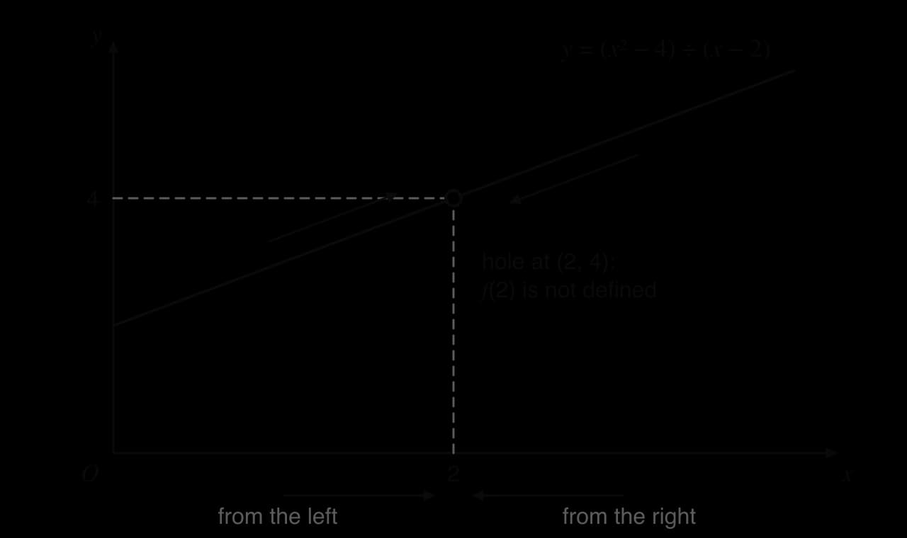
As $x$ gets closer to $2$, from either side, $f(x)$ gets closer to $4$. The value $4$ is the limit of $f(x)$ as $x$ tends to $2$. The reason is visible after factorising: for $x \neq 2$,

so the graph is the straight line $y = x + 2$ with a single point missing at $(2, 4)$.

Two features of the definition matter. First, $x$ approaches $a$ but never equals it, so the value of $f(a)$, or whether $f(a)$ exists at all, makes no difference to the limit. Second, $x$ can approach $a$ from values less than $a$ (from the left) and from values greater than $a$ (from the right). For the limit to exist, both approaches must lead to the same value.

For most familiar functions, such as polynomials, the limit as $x \to a$ is simply $f(a)$, because the graph has no breaks or holes. For example, $\lim_{x \to 3} (x^2 + 1) = 10$. Limits become interesting, and necessary, exactly when direct substitution fails, which is what happens when the gradient of a curve is found.

Estimating a limit from a table

When a limit cannot be found by simplifying, a table of values gives a good estimate. Choose values of $x$ that get steadily closer to $a$ from both sides, such as $a \pm 0.1$, $a \pm 0.01$ and $a \pm 0.001$, and look for the value that $f(x)$ settles on.

A table gives strong evidence for a limit, but it is not a proof: it only shows a few values. The algebraic methods of later subtopics confirm limits exactly. In practice a table is a reliable way to estimate a limit, especially with a GDC.

Limits that do not exist

Not every function has a limit at every point. If the values of $f(x)$ grow without bound, or approach different values from the two sides, there is no limit.

Limits also describe what happens as $x$ grows without bound, written $x \to \infty$. For example, $\frac{1}{x} \to 0$ as $x \to \infty$, which is the horizontal asymptote $y = 0$ of the reciprocal function (2.8). The sum to infinity of a geometric series in 1.8 is a limit of the same kind: $S_\infty$ is the value that $S_n$ approaches as $n \to \infty$.

From chords to tangents

The gradient of a curve at a point

A curve has no single gradient, but at each point it has a direction. The straight line that just touches the curve at a point, going in the same direction as the curve there, is the tangent at that point. The gradient of the curve at the point is defined to be the gradient of this tangent.

A tangent can cross the curve somewhere else, and at some points it even crosses the curve at $P$ itself, so "touches the curve at one point only" is not a correct description. What matters is that, very close to $P$, the curve and the tangent are almost indistinguishable. Zooming in on a smooth curve at any point makes it look more and more like a straight line, and that line is the tangent.

Chord gradients tending to the tangent gradient

The gradient of a tangent cannot be calculated directly from the gradient formula, because only one point on it, $P$, is known. The way round this is to take a second point $Q$ on the curve, find the gradient of the chord $PQ$, and then move $Q$ closer and closer to $P$. As $Q$ approaches $P$, the chord turns towards the tangent, and its gradient approaches the gradient of the tangent.

For the curve $y = x^2$ and the point $P(1, 1)$, take $Q(x, x^2)$. The gradient of the chord $PQ$ is

which cannot be evaluated at $x = 1$, because it gives $\frac{0}{0}$. This is exactly a limit problem: the gradient of the tangent is

The general chord

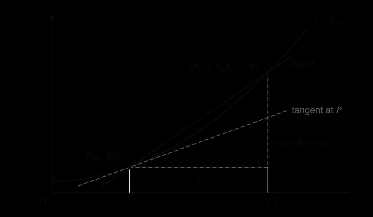
The same method works at any point on any smooth curve. Let $P$ be the point $(a, f(a))$, and let $Q$ be a second point a small horizontal distance $h$ away, at $(a + h, f(a + h))$. The run from $P$ to $Q$ is $h$, and the rise is $f(a + h) - f(a)$.

The gradient of the chord is

and the gradient of the curve at $P$ is the limit of this as $h \to 0$. Here $h$ may be positive ($Q$ to the right of $P$) or negative ($Q$ to the left). Using this limit algebraically, called differentiation from first principles, is part of 5.12 (HL); at this stage the limit is estimated numerically, and from 5.3 onwards it is found with rules.

The derivative

The gradient function

Repeating the chord method at other points on $y = x^2$ gives the gradient of the curve at each of them.

The gradient at each point is twice the $x$-coordinate. The gradient of $y = x^2$ is therefore given by a new function, $2x$. This function is called the gradient function, or the derivative, of $x^2$.

The two graphs are different representations of the same information. At $x = -2$ the parabola is falling steeply and the gradient function has the value $-4$; at $x = 0$ the parabola is momentarily flat and the gradient function is $0$; at $x = 1.5$ the parabola is rising and the gradient function is $3$. How the shape of a graph is related to the sign of its derivative is developed in 5.2.

Notation for the derivative

There are two main notations, and both are used throughout the course.

The notation $\frac{dy}{dx}$, due to Leibniz, recalls how the derivative is made: $dy$ suggests a very small change in $y$ and $dx$ a very small change in $x$. It is a single symbol, not a fraction, so the $d$s cannot be cancelled. Its advantage is that it names both variables, which matters when the variables are not $x$ and $y$: for the volume $V$ of a sphere of radius $r$, the rate of change of volume with respect to radius is $\frac{dV}{dr}$.

Instantaneous rate of change

The gradient of a chord is an average rate of change, and the gradient of the tangent is its limit. In a context, the derivative is therefore the instantaneous rate of change: the rate at a single moment, or at a single value of the input. A car's speedometer shows instantaneous speed, the derivative of distance with respect to time, while dividing the length of a journey by its time gives only the average speed.

Estimating gradients numerically

From a formula: chords on one side or both sides

The chord method gives estimates of a gradient that improve as $h$ gets smaller. A chord from $a$ to $a + h$ lies to one side of the point. A better estimate, for the same value of $h$, uses a chord with one end on each side of the point, from $a - h$ to $a + h$:

On a curve that bends, the one-sided chord is too steep on one side and not steep enough on the other, and the central chord balances the two errors.

From real data

When a quantity is known only from data, a gradient can still be estimated with a chord between neighbouring data points, preferably one on each side of the point of interest. The annual mean carbon dioxide concentration at Mauna Loa was $411.65$ ppm in 2019 and $416.41$ ppm in 2021 (NOAA). The central chord estimate for the rate of increase in 2020 is

compared with an average rate of $0.877$ ppm per year over 1960–1970. The estimate is only as good as the data: a measurement error of a few hundredths of a ppm would barely change it, but data recorded every ten years would give a much rougher value.

From a graph

To estimate the gradient of a curve at a point from its graph, draw the tangent at the point by eye with a ruler, then pick two points on the tangent that are far apart and easy to read. The gradient of the tangent, rise divided by run, estimates the gradient of the curve.

A tangent drawn by eye is only approximate, so an estimate from a graph is usually good to one or two significant figures. Choosing points on the tangent that are far apart reduces the effect of reading errors.

With a GDC

A graphic display calculator (GDC) estimates the gradient of a curve at a point numerically, using a very small central chord. On a graph screen, a "derivative at a point" (often written $\frac{dy}{dx}$) option traces the curve and shows the gradient; in calculations, a numerical derivative function takes the function, the variable and the value of $x$. The answer is a decimal approximation, normally accurate to many significant figures.

Rates of change in context

Units of a derivative

In a context, $\frac{dy}{dx}$ is measured in units of $y$ per unit of $x$, just like an average rate of change. Reading the units from the variables is the first step in interpreting any derivative.

For a sphere, $V = \frac{4}{3}\pi r^3$. A central chord at $r = 3$ cm with $h = 0.001$ gives $\frac{dV}{dr} \approx 113.1$ cm³ per cm, which is $36\pi$, the surface area of the sphere. Increasing the radius by a small amount adds a thin shell to the sphere whose volume is about the surface area times the thickness, which is why the two match.

Interpreting the sign and the size

The sign of a derivative shows the direction of change and its size shows how fast the change happens.

• $\frac{dy}{dx} > 0$: $y$ is increasing as $x$ increases.

• $\frac{dy}{dx} < 0$: $y$ is decreasing as $x$ increases.

• $\frac{dy}{dx} = 0$: $y$ is momentarily not changing.

• A larger value of $\left|\frac{dy}{dx}\right|$

Exam-style questions on limits and the derivative

The second question is set in a context and uses a GDC.

Self-check

• To do:

  I can estimate $\lim_{x \to a} f(x)$ from a table of values on both sides of $a$ and from a graph.

• To do:

  I can explain why a function can have a limit at a point where it is not defined, and recognise limits that do not exist.

• To do:

  I can find the average rate of change of a function over an interval as the gradient of a chord, with units.

• To do:

  I can explain how chord gradients tend to the gradient of the tangent, and use a table of chord gradients to estimate a gradient.

• To do:

  I can describe the derivative as the gradient function and as an instantaneous rate of change.

• To do:

  I can use and read the notations $f'(x)$, $f'(a)$, $\frac{dy}{dx}$

• To do:

  I can estimate the gradient of a curve at a point from a graph, from a central chord and with a GDC.

• To do:

  I can interpret the sign, size and units of a derivative in context.

The point $\mathrm{Q}(1 + h, 2^{1+h})$, where $h > 0$, also lies on the curve. The gradient of the chord $[\mathrm{PQ}]$ is $m$.

The following table shows some values of $h$ and the corresponding values of $m$, correct to five significant figures.

1. (a)

   Use your GDC to find $p$ and $q$.

   [2]2 marks

   Markscheme (a)

   attempt to substitute $h = 0.01$ or $h = 0.001$ into $m = \dfrac{2^{1+h} - 2}{h}$ (M1)

   $p = 1.3911$, $q = 1.3868$ A1

   Note: Accept $p = 1.39$ and $q = 1.39$, or more accurate values ($1.39111\ldots$, $1.38677\ldots$).

2. (b)

   Hence write down an estimate for the gradient of the tangent to the curve at P.

   [1]1 mark

   Markscheme (b)

   $1.39$ (accept $1.386$ or $1.387$) A1

   Note: Award A1 for any value between $1.386$ and $1.390$ inclusive that follows the trend in the table.

3. (c)

   Use your answer to part (b) to find the equation of the tangent to the curve at P. Give your answer in the form $y = ax + b$.

   [2]2 marks

   Markscheme (c)

   attempt to substitute $(1, 2)$ and their gradient into the equation of a straight line (M1)

   $y - 2 = 1.39(x - 1)$

(b) From the right, $\frac{1}{x}$ grows without bound ($10, 100, 1000, \ldots$); from the left, it decreases without bound ($-10, -100, -1000, \ldots$). There is no limit.

(c) For $x > 1$, $|x - 1| = x - 1$, so the expression equals $1$. For $x < 1$, $|x - 1| = -(x - 1)$, so the expression equals $-1$. The values approach $1$ from the right and $-1$ from the left. They do not approach a single value, so the limit does not exist.

(b) With $Q$ to the left of $P$:

(c) From the right the chord gradients decrease towards $2$, and from the left they increase towards $2$. The gradient of the curve at $P$ is $2$.

The tables also show a pattern: when $Q$ has $x = 1 + h$, the chord gradient is $2 + h$. As $h \to 0$, this tends to $2$.

(b) Average speed $= \dfrac{4.9(2 + h)^2 - 19.6}{h}$.

For example, with $h = 0.1$: $s(2.1) = 4.9 \times 4.41 = 21.609$, so the average speed is $\frac{21.609 - 19.6}{0.1} = 20.09$ m s⁻¹.

(c) The average speeds approach $19.6$, so the speed at $t = 2$ is $19.6$ m s⁻¹. In derivative notation,

The average speed over the first full second after $t = 2$, $24.5$ m s⁻¹, is larger because the stone keeps speeding up.

The gradient of the curve at $P$ is $-2$. It is negative because the curve is going down from left to right at $P$: as $x$ increases past $2$, $y$ decreases, at first by about $2$ units for each unit of $x$.

Check with a central chord: $\frac{8/2.01 - 8/1.99}{0.02} = \frac{3.980099 - 4.020101}{0.02} = -2.00005$, which agrees.

A check with a central chord: $\frac{\sqrt{4.001^2 + 9} - \sqrt{3.999^2 + 9}}{0.002} = 0.8000\ldots$. (The exact value, $\frac{4}{5}$, can be found with the chain rule in 5.6.)

as given (M1 for the gradient formula with these values). Every step towards the given answer must be shown.

(b) $1.01^3 = 1.030301$, so

(c) The chord gradients approach $3$, so $f'(1) = 3$.

(d) A half-turn about the origin maps $P(1, 1)$ to $(-1, -1)$ and maps the tangent at $P$ to the tangent at $(-1, -1)$. A half-turn maps a line to a parallel line, so the two tangents have the same gradient: $f'(-1) = 3$.

(c) Using the numerical derivative on the GDC, $N'(10) = 3093.11\ldots \approx 3090$. Ten days after the launch, the total number of downloads is increasing at a rate of about $3090$ downloads per day.

(d) $N'(20) = 1448.61\ldots \approx 1450$ downloads per day. By day $20$ about $44\,600$ of the $50\,000$ downloads predicted by the model have happened, so there are fewer new users left to download the app and the rate of downloading has slowed down.

$y = 1.39x + 0.61$ (accept $y = 1.386x + 0.614$) A1FT

Note: Follow through from their answer to part (b).

• y = f(x)

Find the value of $f(0.01)$.

[1]1 mark

Show that the gradient of the chord $[\mathrm{PQ}]$ is $1 - h$.

[2]2 marks