2.11 Market failure: market power

Analyse how firms with market power set price and output, draw every market structure diagram, calculate costs, revenues and profit, and evaluate large firms and government responses to their power.

IB Economics
Part of 2 Microeconomics
HL only

Key terms introduced here

Each is in the Economics glossary, with every other term in the subject.

Abnormal profit: Profit above normal profit, earned when total revenue exceeds total economic cost, or when average revenue is greater than average cost (AR > AC).
Average cost: Total cost per unit of output, found by dividing total cost by the quantity produced (AC = TC ÷ Q); also called average total cost.
Average revenue: Total revenue per unit sold, found by dividing total revenue by the quantity sold (AR = TR ÷ Q); it equals the price, so the AR curve is the firm's demand curve.
Average variable cost: Total variable cost per unit of output, found by dividing total variable cost by the quantity produced (AVC = TVC ÷ Q).
Barriers to entry: Obstacles that make it difficult or impossible for new firms to enter a market, such as economies of scale, patents, licences, control of key resources or strong brand loyalty.
Cartel: A formal agreement between firms, or countries, to act together as if they were a single monopoly, usually by fixing prices or setting output quotas.
Collusion: An agreement, formal or informal, between firms in a market to limit competition, for example by fixing prices, limiting output or sharing out customers.

Carry on with 2.11 in Augment

With a free account, Augment remembers where you stopped and what you have practiced.

Start free Open 2.11 in Augment

2.11 Market failure: market power · IB Economics | Augment Education

Notes on 2.11 Market failure: market power

71 min readLast reviewed 14 Oct 2026

Learning objectives

Describe the four market structures and the barriers to entry that separate them.
Calculate total, average and marginal costs and revenues, and profit, from data.
Explain why profit is maximised where MC = MR, and identify abnormal profit, normal profit and losses on a diagram.
Draw and explain diagrams of a perfectly competitive firm in the short run and the long run, and of allocative efficiency in a competitive market.
Draw and explain diagrams of monopoly profit, natural monopoly and the welfare loss of monopoly compared with perfect competition.
Explain collusive and non-collusive oligopoly using a collusive oligopoly diagram, a payoff matrix and concentration ratios.
Draw and explain the short-run and long-run diagrams of monopolistic competition, and compare its demand curve with that of a monopoly.
Evaluate the advantages and risks of markets dominated by large firms with significant market power.
Evaluate legislation and regulation, government ownership and fines as responses to the abuse of market power.

Introduction

Market power is the ability of a firm to influence the price of what it sells. Markets range from those where no single firm has any influence over price, such as the world market for wheat, to those dominated by one firm or a handful of firms, such as search engines, aircraft manufacturing or crude oil, where a single decision can move prices around the world.

When firms have significant market power, they can restrict output and raise price above the cost of producing the last unit, so the market produces less than society wants. This is a form of market failure, and it raises questions about efficiency (resources are misallocated), equity (consumers pay more and owners of the firm gain) and intervention (whether, and how, governments should limit the power of large firms).

Market structures

Economists group markets by their market structure: the features that shape how firms in a market behave. The most important features are the number and size of firms, whether their products are identical or different, how easily new firms can enter the market, and how much control each firm has over price.

Four structures are used to analyse almost every real market. They sit on a spectrum from no market power at one end to complete market power at the other.

Perfect competition

In perfect competition, a very large number of small firms sell an identical product. Each firm’s output is so small compared with the whole market that it cannot affect the market price, and new firms can enter (or existing firms leave) freely. Buyers and sellers have full information about prices and quality.

A homogeneous product is one that buyers regard as identical whoever makes it: one tonne of a given grade of wheat is the same as any other. Because buyers have no reason to prefer one seller, a firm that tried to charge more than the market price would sell nothing.

Monopoly

At the other end of the spectrum, a monopoly is a market supplied by a single firm, or one firm so dominant that it controls the market. The product has no close substitutes, so buyers who want it must buy from the monopolist, and high barriers to entry stop other firms from competing the abnormal profit away.

A monopoly can keep abnormal profit in the long run only because rivals cannot get in. What stops them is a barrier to entry.

Imperfect competition: oligopoly and monopolistic competition

Most real markets lie between the two extremes and are described as imperfect competition. Firms in these markets have some market power, but less than a monopoly. Two structures are distinguished.

Oligopoly: a few large firms dominate the market, protected by high barriers to entry. Products may be identical (oil, steel, cement) or differentiated (cars, smartphones, soft drinks). Because there are only a few firms, each one’s decisions affect the others, so the firms are interdependent.
Monopolistic competition: many firms sell products that are slightly different from each other, and entry and exit are free. Cafés, hairdressers, restaurants and clothing shops are typical examples. Each firm has a small amount of market power because its product is not quite the same as its rivals’.

Product differentiation is what gives a monopolistically competitive firm its market power. A café can charge a little more than the one next door because its location, coffee, atmosphere or brand are slightly different, and some customers prefer them.

Feature	Perfect competition	Monopolistic competition	Oligopoly	Monopoly
Number of firms	Very many, all small	Many	A few large firms dominate	One (or one dominant firm)
Product	Homogeneous (identical)	Differentiated	Homogeneous or differentiated	Unique, no close substitutes
Barriers to entry	None	None or very low	High	Very high
Control over price	None (price taker)	Some (price maker)	Considerable, but interdependent	Considerable (price maker)
Long-run profit	Normal profit	Normal profit	Abnormal profit possible	Abnormal profit possible
Examples	Wheat, some fruit and vegetable markets	Cafés, hair salons, restaurants	Crude oil, supermarkets, mobile networks, trucks	Water supply, patented medicines, national rail networks

Where barriers to entry come from

Barriers to entry explain why market power can last. Without them, abnormal profit would attract new firms, and their extra supply would push the price down. The main barriers are the following.

Economies of scale: when average cost falls as output rises, a large established firm can produce more cheaply than any small newcomer, which would make losses while it grew.
Legal barriers: a patent gives an inventor the sole right to make and sell a new product, usually for 20 years; licences and franchises granted by the government (for example to run a railway line or a broadcasting service) exclude other firms by law.
Control of essential resources: a firm that owns the main source of a raw material, or the only network (pipes, cables, rails), can stop others from producing.
Brand loyalty and advertising: years of advertising create strong brands that a newcomer can only match with very large spending.
High start-up costs and sunk costs: building a steel plant, an aircraft factory or a mobile network costs billions, and much of this cannot be recovered if the entrant fails.
Network effects: some products, such as social networks and payment systems, become more useful the more people use them, so the largest network attracts ever more users.
Anti-competitive behaviour: established firms may cut prices temporarily to drive out newcomers, or sign exclusive contracts with suppliers and retailers.

Costs of production

To understand how a firm chooses its output and price, both sides of its decision are needed: what each level of output costs, and what revenue it brings in. Costs come first.

Economists distinguish two time periods. In the short run, at least one factor of production is fixed: a factory cannot be built or extended in a week, so the firm can raise output only by adding variable factors such as labour and materials to its existing capital. In the long run, all factors are variable, so the firm can change its scale of production.

Total, fixed and variable costs

In the short run, a firm’s total cost is made up of two parts. Fixed costs do not change with output: rent, insurance, interest on loans and the salaries of permanent managers must be paid whether the firm produces nothing or runs at full capacity. Variable costs rise as output rises, because more output needs more raw materials, energy and hours of labour.

Fixed costs exist only in the short run: in the long run the firm can end a lease or sell a building, so every cost becomes variable.

\text{Total cost (TC)} = \text{total fixed cost (TFC)} + \text{total variable cost (TVC)}

Average and marginal costs

Cost per unit is often more useful than total cost, because it can be compared directly with the price. Average cost (AC, also called average total cost) is total cost divided by output. It is the sum of average variable cost (AVC) and average fixed cost (AFC).

\text{AC} = \frac{\text{TC}}{Q} \qquad \text{AVC} = \frac{\text{TVC}}{Q} \qquad \text{AFC} = \frac{\text{TFC}}{Q} \qquad \text{AC} = \text{AVC} + \text{AFC}

Marginal cost (MC) is the extra cost of producing one more unit of output. When output changes by more than one unit, it is the change in total cost divided by the change in output. Because fixed costs do not change, marginal cost depends only on variable costs.

\text{MC} = \frac{\Delta \text{TC}}{\Delta Q}

The shapes of the short-run cost curves

Short-run marginal cost first falls and then rises. As the first workers are added to a fixed amount of capital, they can specialise, so each extra worker adds more output than the one before and the cost of each extra unit falls. Beyond some point, the law of diminishing marginal returns sets in: each extra worker has less capital to work with, adds less output, and so each extra unit costs more. This is why the MC curve is shaped like a tick.

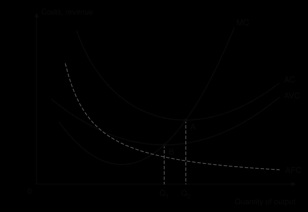
Short-run cost curves of a firm: costs on the vertical axis, quantity of output on the horizontal. A U-shaped MC curve cuts AVC at its minimum point B (output Q1) and AC at its minimum point A (output Q2). AFC is a dashed curve falling throughout. — MC cuts both AVC and AC at their minimum points (B and A). AFC falls throughout, because the same fixed cost is spread over more units, so the gap between AC and AVC narrows as output rises.

The AVC and AC curves are U-shaped. They fall while marginal cost is below them and rise once marginal cost is above them, so the MC curve passes through the lowest point of each. The gap between AC and AVC is average fixed cost, which keeps shrinking as output increases.

Long-run costs: economies and diseconomies of scale

In the long run a firm can change all its inputs, including the size of its factories. The long-run average cost (LRAC) curve shows the lowest average cost at which each level of output can be produced when the firm is free to choose its scale. Its shape is explained by economies of scale and diseconomies of scale, not by diminishing returns, which apply only in the short run.

Large firms gain economies of scale in several ways.

Technical: large plants can use specialised machinery and production lines that would be too expensive for a small firm; doubling the size of a container ship or a storage tank much less than doubles its cost.
Specialisation: in a large firm, workers and managers can specialise in narrow tasks and become more productive.
Purchasing (bulk buying): large buyers negotiate lower prices for materials and components.
Financial: large firms are seen as less risky, so they borrow at lower interest rates and can raise money by issuing shares.
Marketing: the cost of a national advertising campaign is spread over many more units.
Risk-bearing: a firm selling many products in many countries is less exposed to a fall in demand in any one of them.

Beyond some size, a firm may find that average cost starts to rise again. Very large organisations are harder to coordinate, communication between departments slows down, decisions take longer, and workers may feel less motivated in a firm where they have little contact with the people making decisions.

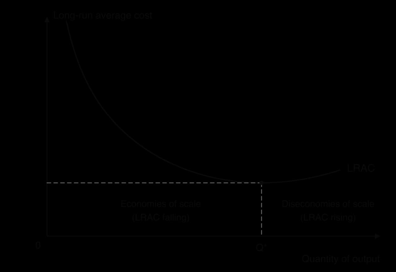
A U-shaped long-run average cost (LRAC) curve. LRAC falls as output rises (economies of scale) to a minimum at output Q*, then rises (diseconomies of scale). — LRAC falls while economies of scale outweigh diseconomies, reaches its minimum at Q*, then rises. Where Q* lies compared with total market demand decides how many firms the market can support.

How far economies of scale extend compared with the size of the market has a large effect on market structure. If LRAC reaches its minimum at a small output, many firms can each produce at the lowest cost, and competition is likely. If LRAC keeps falling up to an output close to the whole market’s demand, only a few firms, or even one, can survive. This is the source of the natural monopoly, analysed later.

Revenue

A firm’s revenue is the money it receives from selling its output. Total revenue (TR) is the price multiplied by the quantity sold. As with costs, two other measures are used: average revenue (AR), the revenue per unit sold, and marginal revenue (MR), the extra revenue from selling one more unit.

\text{TR} = P \times Q \qquad \text{AR} = \frac{\text{TR}}{Q} = P \qquad \text{MR} = \frac{\Delta \text{TR}}{\Delta Q}

Marginal revenue looks at the change at the margin: how much the last unit sold added to total revenue.

Revenue curves of a price taker

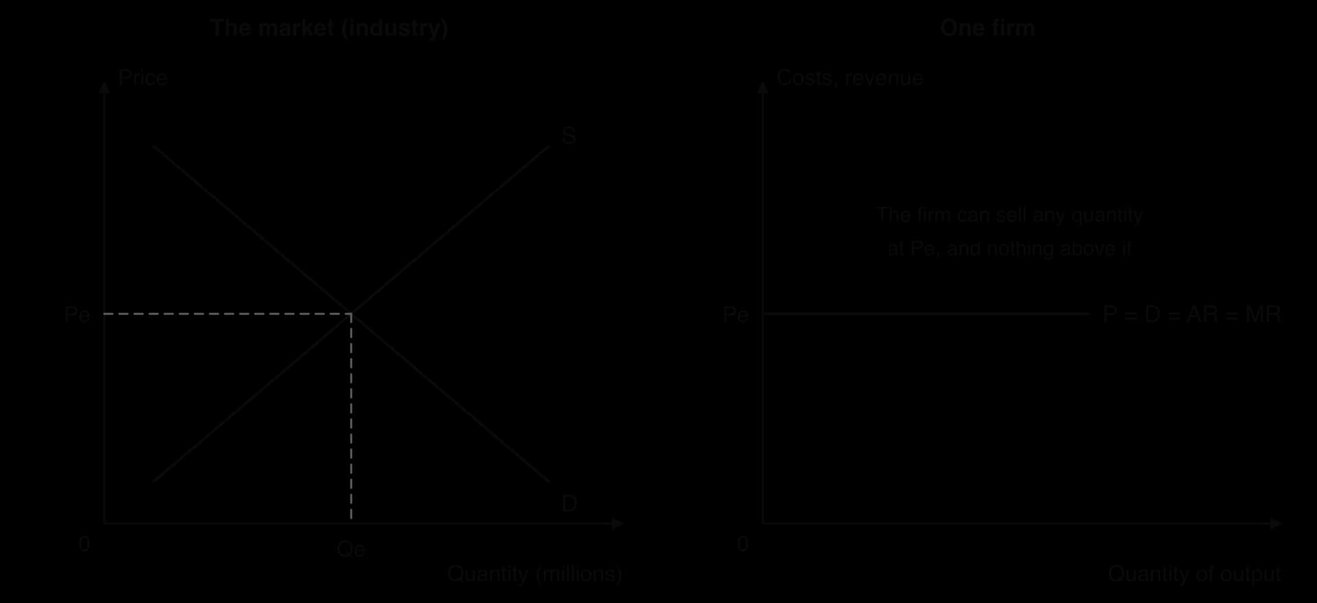
A firm in perfect competition is a price taker: it must accept the market price. It can sell as much as it wants at that price, but nothing at all at a higher price, because buyers would go to one of the many identical sellers. Its demand curve is therefore horizontal (perfectly elastic) at the market price.

Since every unit sells at the same price, each extra unit adds exactly that price to total revenue. For a price taker, price, average revenue and marginal revenue are all the same, and the firm’s demand curve is labelled P = D = AR = MR.

Revenue curves of a price maker

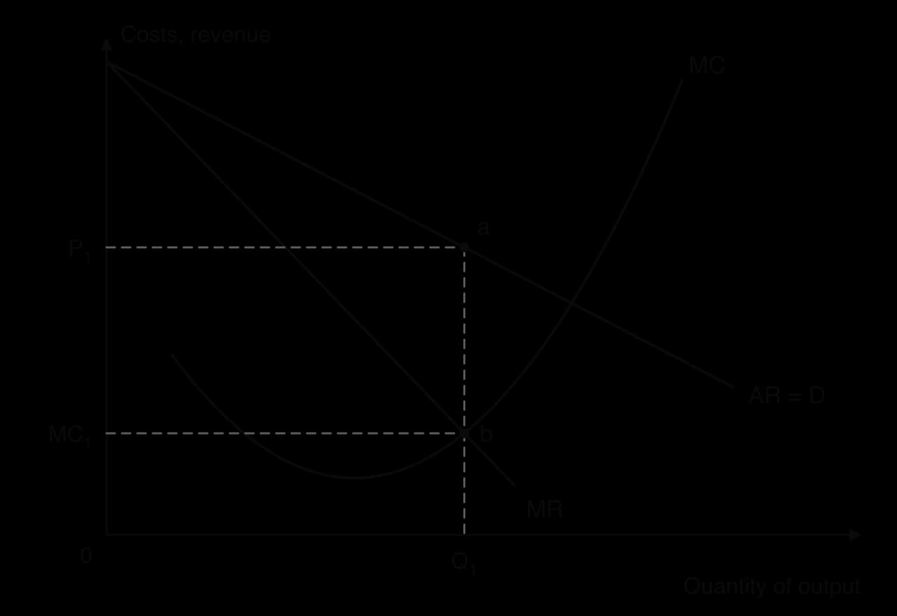
A firm with market power faces the downward-sloping demand curve of its own product, so it is a price maker. It can choose its price, but then the demand curve decides how much it sells; or it can choose its output, and the demand curve decides the price. It cannot choose both.

For a price maker, marginal revenue is less than price. To sell one more unit, the firm must lower its price, and (assuming it charges everyone the same price) the lower price applies to all the units it was already selling, not just the extra one. The extra unit adds its own price to revenue, but the firm loses revenue on all the other units.

With a straight-line demand curve, the MR curve starts at the same point on the price axis and falls twice as steeply, so it cuts the quantity axis halfway to where the demand curve does. Marginal revenue is positive where demand is price elastic, zero where price elasticity of demand (PED) equals 1, and negative where demand is inelastic. Where MR is negative, selling more units actually reduces total revenue.

Revenue curves of a price maker: a downward-sloping AR = D line and an MR line from the same vertical intercept, twice as steep, reaching zero at Q1, where PED = 1 on AR at price P1. Demand is elastic above P1 and inelastic below it. — MR shares AR’s vertical intercept and is twice as steep, reaching zero at Q₁, where PED = 1. Above P₁ demand is elastic and MR is positive; below it MR is negative.

Since marginal cost is always positive, a profit-maximising firm never produces where MR is negative. A firm with market power therefore always sets its price in the elastic part of its demand curve.

Profit maximisation

Standard theory assumes that firms aim at profit maximisation: they choose the output that makes the difference between total revenue and total cost as large as possible. Other objectives, such as growth, market share or social responsibility, are real, but profit maximisation is the starting point that explains most of how firms respond to changes in costs and demand.

\text{Profit} = \text{TR} - \text{TC}

Normal profit, abnormal profit and losses

Because economic costs include opportunity costs, a firm that just covers all its costs is still earning a return on the owner’s time and capital equal to what they could earn in their next best use. This minimum return is called normal profit, and it is counted as a cost.

Any profit above this is abnormal profit (sometimes called supernormal or economic profit). If revenue does not cover all economic costs, the firm makes a loss. Comparing average revenue with average cost at the chosen output shows which of the three a firm is earning.

Abnormal profit is a signal: it shows that resources earn more in this market than elsewhere, which attracts new firms if they can enter.

Comparison at the chosen output	Total values	What the firm earns	What happens in the long run (without barriers to entry)
AR > AC	TR > TC	Abnormal profit	New firms are attracted into the market
AR = AC	TR = TC	Normal profit	No incentive to enter or leave
AR < AC	TR < TC	Loss	Some firms leave the market

Why profit is maximised where MC = MR

The profit-maximising output can be found by marginal reasoning. A firm compares what one more unit adds to revenue (MR) with what it adds to cost (MC).

If MR > MC, producing the extra unit adds more to revenue than to cost, so profit rises. The firm should expand output.
If MR < MC, the last unit added more to cost than to revenue, so profit fell. The firm should cut output.
Only where MR = MC can profit not be increased by changing output. This is the profit-maximising output.

The rule holds in every market structure, which is what makes it so useful. The differences between the structures come from the shapes of the revenue curves, not from a different rule. The MC curve must cut MR from below: where MC is still falling, the firm could raise profit by producing more.

The table gives hypothetical price and cost data for a firm with market power, with output in units per day. It is used in the worked example that follows.

Output (Q)	0	1	2	3	4	5	6
Price (AR) ($)	22	20	18	16	14	12	10
Total cost (TC) ($)	12	15	20	27	36	47	60

Using the hypothetical data in the table, calculate the firm’s marginal revenue, marginal cost, average cost and profit at each output, and determine the profit-maximising output and price.

Show the solution

Step 1: total revenue. TR = P × Q for each output: 0, 20, 36, 48, 56, 60, 60.

Step 2: marginal revenue and marginal cost. Each is the change from the previous output. MR: 20, 16, 12, 8, 4, 0. MC: 3, 5, 7, 9, 11, 13.

Step 3: average cost and profit. AC = TC ÷ Q and profit = TR − TC.

Q	TR	MR	TC	MC	AC	Profit
0	0	–	12	–	–	−12
1	20	20	15	3	15.00	5
2	36	16	20	5	10.00	16
3	48	12	27	7	9.00	21
4	56	8	36	9	9.00

Reading profit from a diagram

On a diagram, profit (or loss) is a rectangle. Its height is the difference between AR and AC at the profit-maximising output, which is the profit per unit; its width is the quantity sold. In symbols, total abnormal profit = (AR − AC) × Q, and the same expression gives the size of a loss when AR < AC.

Degrees of market power

A firm’s market power depends on how easily its customers can switch to substitutes. The more close substitutes there are, the more elastic the demand for the firm’s product, and the less it can raise its price without losing most of its sales.

A useful sign of market power is the gap between price and marginal cost. A price taker sells at a price equal to its marginal cost. A firm with market power restricts output to the point where MC = MR, and since MR is below the price for a price maker, the price it charges (AR) is above its marginal cost. The larger the gap between AR and MC, the more market power the firm has.

Price maker with MC, AR = D and MR. MC = MR at point b, output Q1, where marginal cost is MC1. The price read from AR at Q1 is P1 (point a), well above MC1: price is greater than marginal cost. — At the profit-maximising output Q₁ (point b, MC = MR), the firm charges P₁ (point a) on its demand curve. The vertical gap between a and b shows market power: price exceeds marginal cost.

Structure	Market power	Demand curve facing the firm	Price compared with MC
Perfect competition	None: price taker	Horizontal (perfectly elastic)	P = MC
Monopolistic competition	Low: price maker	Downward sloping and quite elastic	P slightly above MC
Oligopoly	High, but limited by rivals’ reactions	Downward sloping; depends on rivals	P well above MC (especially with collusion)
Monopoly	Highest	The market demand curve, less elastic	P well above MC

Perfect competition

Perfect competition is a model, and few real markets meet all its conditions. Its value is as a benchmark: it shows what a market with no market power at all would achieve, so that the outcomes of the other structures can be measured against it.

The assumptions of the model

Very many small firms and buyers: each supplies or buys a tiny share of the market, so none can affect the price.
A homogeneous product: every firm’s output is identical, so buyers care only about price.
Free entry and exit: there are no barriers, so firms can enter when there is abnormal profit and leave when they make losses.
Perfect information: all buyers and sellers know the prices charged by every firm and the methods of production available.
Perfect mobility of factors of production: resources can move freely between markets.

Some agricultural markets come close. Thousands of farmers grow wheat of a given grade, no single farm can affect the world price, and a farm that asked more than the market price would find no buyers. Markets for major currencies and for the shares of large companies, with very many buyers and sellers of an identical asset, are also close to the model.

The firm as a price taker

The market price is set by the interaction of market demand and market supply. Each firm takes that price as given and faces a horizontal demand curve at it, because it can sell its entire output at the market price.

Two panels. Left: industry demand D and supply S intersect at price Pe and quantity Qe. Right: a single firm faces a horizontal demand curve at Pe, labelled P = D = AR = MR, so it can sell any quantity at Pe. — Industry demand and supply set the price Pe (left). The firm (right) takes Pe as given: its demand curve is horizontal at Pe, so P = D = AR = MR.

EconplusDal (13 min) on the perfectly competitive firm as a price taker, its short-run profits and losses, the long-run adjustment and efficiency. The video follows UK A-level, but the theory and diagrams are the same.

Short-run profit maximisation

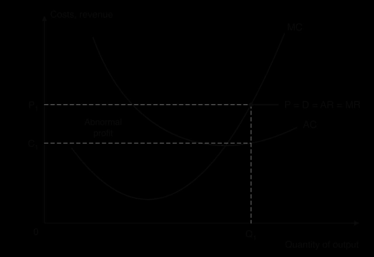
A perfectly competitive firm follows the same rule as any other firm: it produces where MC = MR. Since MR equals the price, this means it produces where its rising MC curve cuts the horizontal price line. Whether it makes abnormal profit, normal profit or a loss depends on where the price lies compared with its average cost.

Abnormal profit in the short run

If the market price P₁ is above the firm’s average cost at the profit-maximising output, the firm earns abnormal profit. At Q₁, average revenue is P₁ and average cost is C₁, so abnormal profit per unit is P₁ − C₁ and total abnormal profit is the shaded rectangle (P₁ − C₁) × Q₁.

Perfectly competitive firm with MC and AC curves and a horizontal P = D = AR = MR line at P1. MC = MR at output Q1, where average cost is C1, below P1. The rectangle between P1 and C1 up to Q1 is shaded as abnormal profit. — MC = MR at Q₁. Price P₁ is above average cost C₁, so the firm earns abnormal profit equal to the shaded rectangle (P₁ − C₁) × Q₁.

Losses in the short run and the shut-down price

If the price falls below average cost, the firm makes a loss at every output. It still chooses the output where MC = MR, because that output keeps the loss as small as possible. The question is whether it should produce at all.

In the short run the firm must pay its fixed costs even if it produces nothing. If it shuts down, its loss equals its total fixed cost. If it produces, it is better off than shutting down as long as its revenue covers its variable costs, because every dollar of revenue above variable cost helps to pay the fixed costs. The firm therefore keeps producing in the short run as long as the price is at least equal to average variable cost. The price equal to minimum AVC is therefore the firm’s shut-down price.

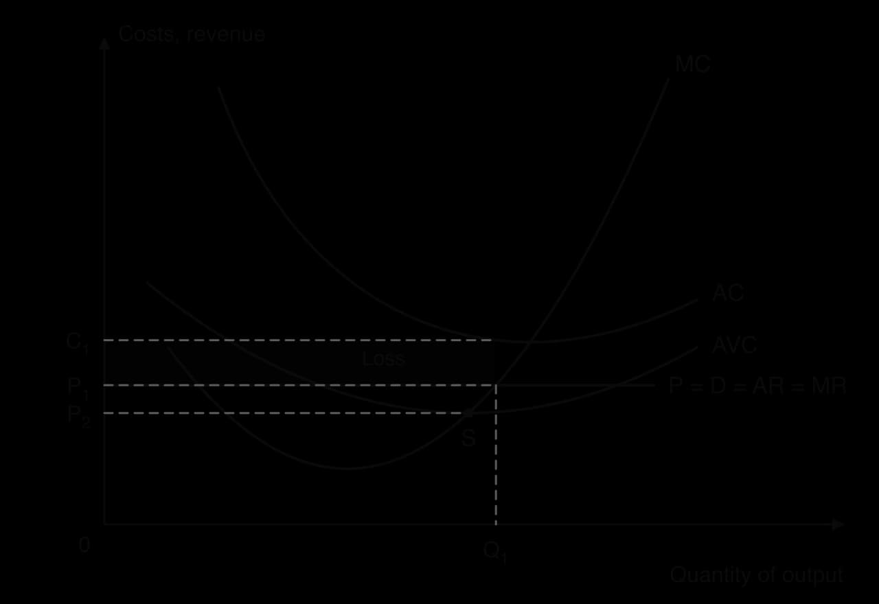
Perfectly competitive firm with MC, AC and AVC curves and a horizontal P = D = AR = MR line at P1, below AC but above AVC. MC = MR at Q1 where AC is C1; the rectangle between C1 and P1 is shaded as a loss. S marks minimum AVC at price P2, the shut-down price. — At P₁ the firm makes a loss (shaded), but P₁ is above AVC, so producing Q₁ loses less than shutting down. S marks minimum AVC: below P₂ the firm should stop producing.

In the long run there are no fixed costs, since all inputs can be changed. A firm that expects to keep making a loss will leave the market: in the long run it must cover all its costs, so the long-run condition for staying in business is P ≥ AC.

The next table gives hypothetical cost data for a perfectly competitive firm with total fixed costs of $20 a day. It is used in the worked example.

Output (Q, units per day)	1	2	3	4	5	6	7
Total variable cost (TVC) ($)	8	14	18	24	32	43	56

Using the hypothetical data in the table (total fixed cost $20), (a) calculate the firm’s profit-maximising output and its profit or loss when the market price is $10; (b) state whether the firm should continue to produce in the short run; (c) determine the shut-down price and explain what the firm does if the price falls to $5.

Show the solution

Step 1: marginal cost and average variable cost. MC is the change in TVC (fixed costs do not change): 8, 6, 4, 6, 8, 11, 13. AVC = TVC ÷ Q: 8.00, 7.00, 6.00, 6.00, 6.40, 7.17, 8.00.

Step 2 (a): output at P = $10. For a price taker MR = P = $10. The fifth unit has MC = $8 < $10, so it adds to profit; the sixth has MC = $11 > $10, so it does not. The firm produces 5 units.

Step 3: profit or loss. TR = 5 × $10 = $50. TC = $20 + $32 = $52. Profit = $50 − $52 = −$2, a loss of $2 a day.

Step 4 (b): keep producing? If the firm shut down, its loss would be its fixed cost of $20. By producing it loses only $2, because the price ($10) is above AVC ($6.40), so revenue covers variable costs and contributes $18 to fixed costs. The firm continues to produce in the short run.

Step 5 (c): shut-down price. Minimum AVC is $6 (at 3 or 4 units), so the shut-down price is $6. At a price of $5, the best the firm can do by producing is a loss of $23 (TR $15, TC $38 at 3 units), which is worse than the $20 it loses by shutting down. It stops producing.

The long run: entry, exit and normal profit

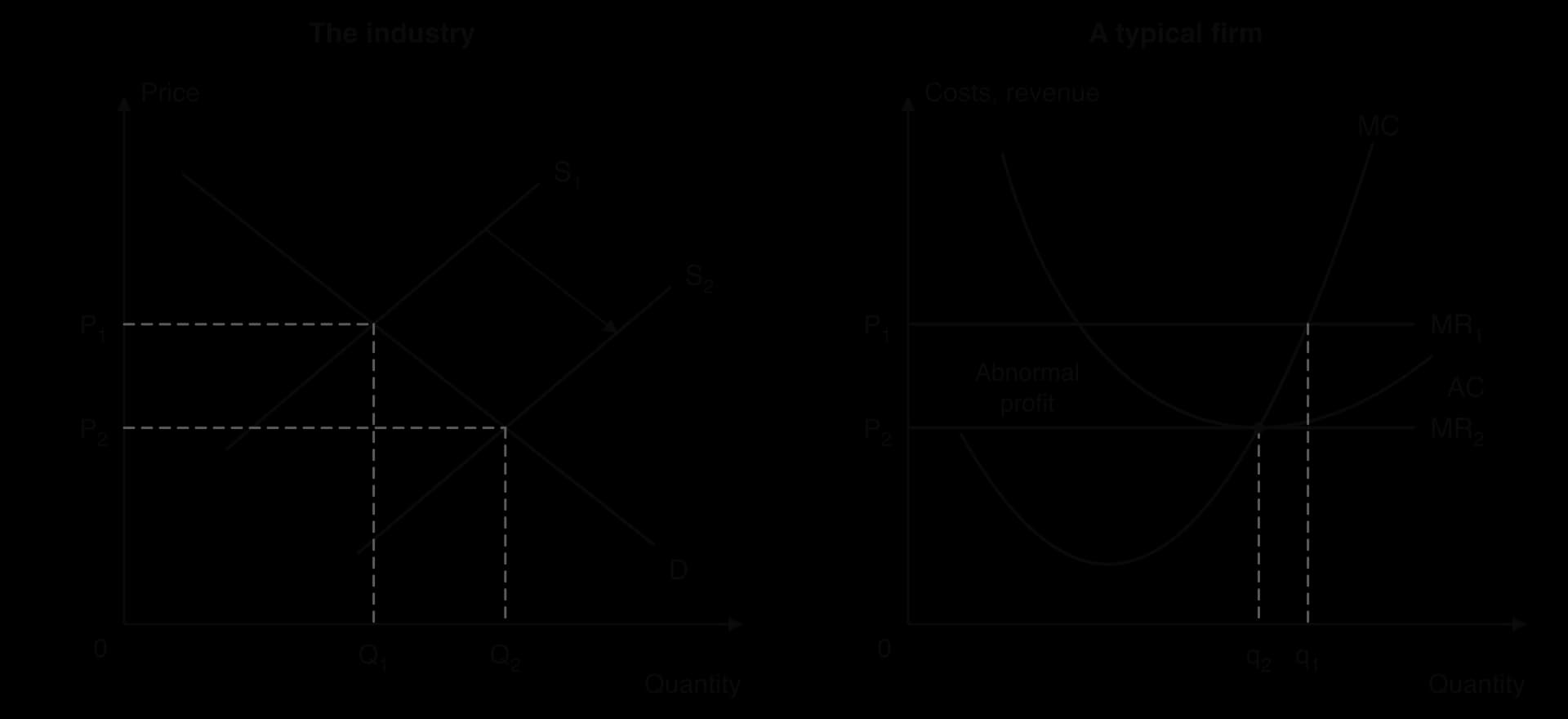
Abnormal profit cannot last in perfect competition. Because there are no barriers to entry and everyone has perfect information, new firms enter the market when existing firms earn abnormal profit. Market supply shifts to the right, the market price falls, and each firm’s horizontal demand curve moves down with it.

Entry continues until the price has fallen to the minimum point of the firms’ average cost curve. There, P = AC, so every firm earns only normal profit, and there is no longer any incentive for new firms to enter.

Two panels. Industry: supply shifts right from S1 to S2 along demand D, price falls from P1 to P2 and quantity rises from Q1 to Q2. Firm: at P1 (MR1) it earns abnormal profit at q1; at P2 (MR2), equal to minimum AC, it earns normal profit at q2. — Abnormal profit at P₁ attracts entry: industry supply shifts from S₁ to S₂ and the price falls to P₂, equal to minimum AC. Each firm cuts output from q₁ to q₂ and earns normal profit.

Losses set off the opposite process. Some firms leave the market, market supply shifts to the left and the price rises until the remaining firms again earn normal profit at the minimum of their average cost.

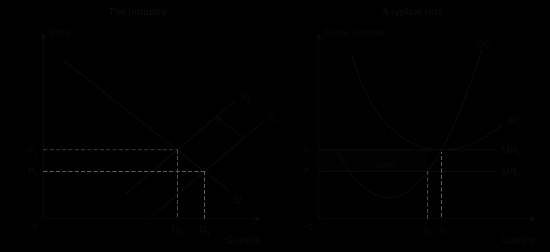
Two panels. Industry: supply shifts left from S1 to S2, price rises from P1 to P2 and quantity falls from Q1 to Q2. Firm: at P1 (MR1) it makes a loss at q1; at P2 (MR2), equal to minimum AC, it earns normal profit at q2. — Losses at P₁ cause exit: industry supply shifts left from S₁ to S₂ and the price rises to P₂ = minimum AC, where the remaining firms earn normal profit at q₂.

In long-run equilibrium, therefore, every perfectly competitive firm produces where

P = \text{AR} = \text{MR} = \text{MC} = \text{minimum AC}

Allocative efficiency in perfect competition

Allocative efficiency means that resources are used to produce the combination of goods and services that society values most. In a single market it is reached when the last unit produced is valued by consumers exactly as much as it costs society to produce, that is, where marginal benefit equals marginal cost (MB = MC).

In a competitive market the demand curve shows the marginal benefit consumers get from each unit, and the supply curve, made up of the firms’ MC curves, shows the marginal cost of producing it. At the market equilibrium, the price equals both, so P = MB = MC. Each firm, by producing where P = MC, produces exactly the quantity at which the value of the last unit to consumers equals its cost.

At this output, social surplus (community surplus), the sum of consumer surplus and producer surplus, is as large as it can be. Producing one unit less would give up a unit that consumers value more than it costs; producing one unit more would use resources worth more than the unit is worth to consumers.

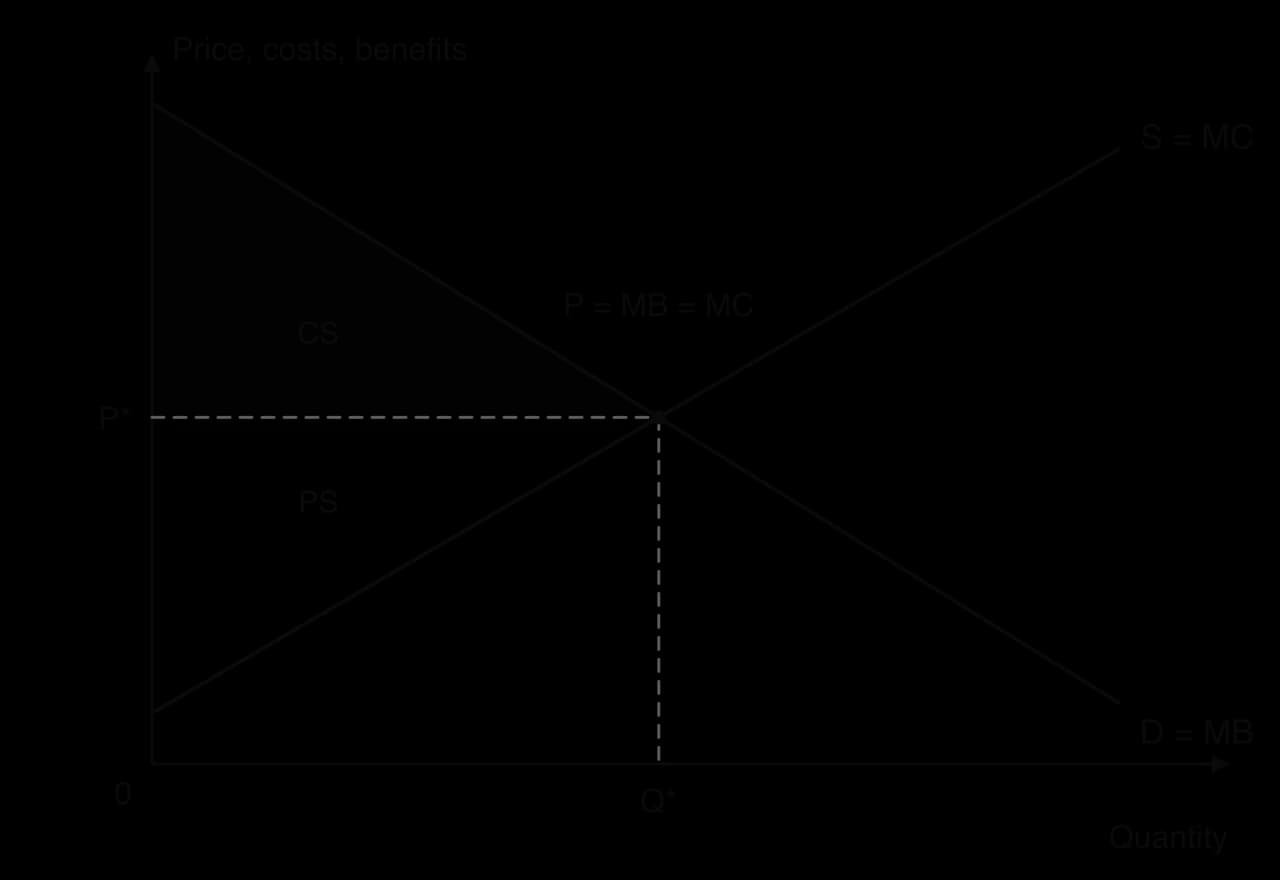
Competitive market: D = MB slopes down and S = MC slopes up, meeting at P* and Q*, labelled P = MB = MC. Consumer surplus (CS) is shaded above P* below D; producer surplus (PS) is shaded below P* above S. — At Q*, P = MB = MC: the value of the last unit to consumers equals its cost. Consumer surplus (CS) plus producer surplus (PS) is maximised, so there is no welfare loss.

Allocative efficiency depends on several conditions: competition strong enough that price equals marginal cost, no externalities (so that private costs and benefits equal social ones), and buyers and sellers with full information. When firms have market power, the first condition fails.

Perfect competition also achieves productive efficiency in the long run: each firm produces at the lowest point of its AC curve, so goods are made at the lowest possible cost per unit and no resources are wasted.

Evaluating perfect competition as a benchmark

The model shows clearly why competition benefits consumers: prices are driven down to the lowest possible average cost, firms that are inefficient are forced out, and resources move to where they are most valued. It is still a theoretical ideal, and its limits matter when it is used to judge real markets.

Unrealistic assumptions: perfect information and identical products are rare; most markets have some branding, location differences or uncertainty about quality.
No economies of scale: in many industries the lowest cost is reached only by large firms, so a market of many tiny firms would have higher costs than one with a few large ones.
Little innovation: with only normal profit in the long run, and with any new idea copied at once under perfect information, firms have neither the funds nor the incentive to spend on research.
No variety: homogeneous products mean consumers have no choice of styles, brands or qualities, which many consumers value.

Monopoly

A pure monopoly, a single seller with no close substitutes, is as rare as perfect competition. In practice, competition authorities treat a firm as having monopoly power, often called a dominant position, when it has a large enough share of a market to act largely independently of competitors and customers. The model of monopoly applies, with some adjustment, to any firm with this kind of power.

Sources of monopoly power

A monopoly keeps its position only as long as barriers to entry keep rivals out. Some barriers arise naturally from the technology of the industry (economies of scale, network effects), some are created by law (patents, licences), and some come from the firm’s own actions (brand building, exclusive contracts, aggressive pricing against entrants).

Patents show the trade-off at the heart of monopoly policy. Gilead Sciences, which owned the patent on the hepatitis C medicine sofosbuvir (sold as Sovaldi), set a US list price of about $84,000 for a 12-week course in 2014, about $1,000 a pill. The company had paid about $11 billion in 2011 to buy the firm that developed the drug, and argued that high prices recover the cost of research; critics pointed to the far lower price, about $300 a course, at which Gilead agreed to sell its own version in India.

Sources: Wikipedia, “Sofosbuvir” (accessed 2026), citing Pharmacy Purchasing & Products and Gilead Sciences.

Profit maximisation by a monopolist

A monopolist is the whole industry, so the market demand curve is its own AR curve, and its MR curve lies below it. It maximises profit where MC = MR, at output Q₁, and sets the highest price consumers will pay for that output, P₁, read from the demand curve.

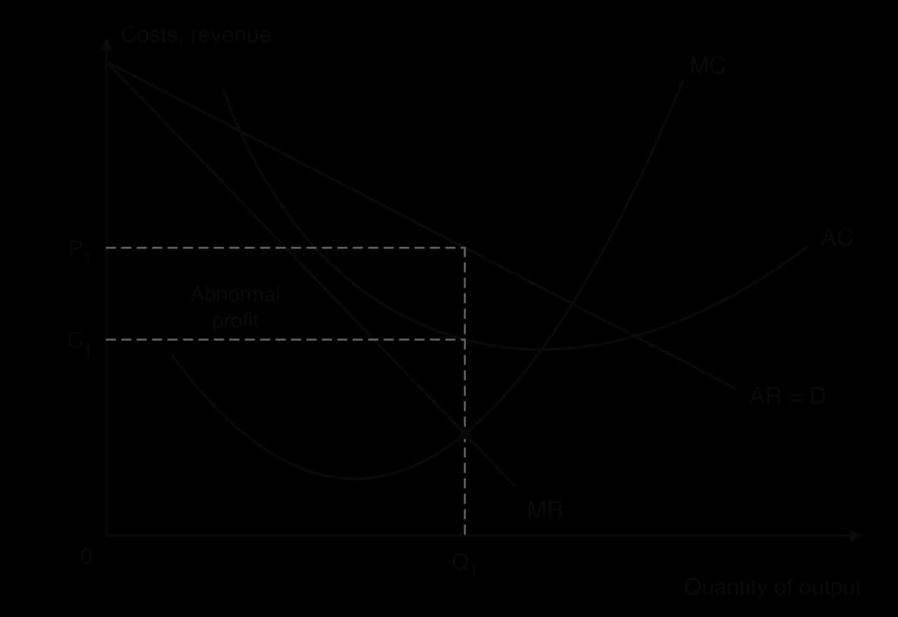
Monopoly with MC, AC, AR = D and MR curves. MC = MR at output Q1; price P1 is read from AR and average cost C1 from AC. The rectangle between P1 and C1 up to Q1 is shaded as abnormal profit. — MC = MR gives output Q₁; the demand curve gives the price P₁. Since P₁ is above the average cost C₁, the monopolist earns abnormal profit (P₁ − C₁) × Q₁, shaded.

Barriers to entry protect this abnormal profit. New firms are attracted by it, but cannot enter, so the monopolist can earn abnormal profit in the long run as well as the short run. This is the main difference in outcome between monopoly and perfect competition.

A monopoly does not always earn abnormal profit. If demand for its product is low compared with its costs, the best it can do may be to cover its costs exactly (normal profit, where AR is tangent to AC) or to keep its loss as small as possible. A monopolist that expects losses to continue will leave the industry in the long run, like any other firm.

Two monopoly panels. Left: AR is tangent to AC at the output Q1 where MC = MR, so price P1 equals average cost (normal profit). Right: at Q1, where MC = MR with MC rising, price P1 is below average cost C1; the rectangle between them is shaded as a loss. — Left: AR just touches AC at the output where MC = MR, so the monopolist earns normal profit (P₁ = AC). Right: AR lies below AC at that output, so it makes the loss shaded, (C₁ − P₁) × Q₁.

Allocative inefficiency and welfare loss

A monopoly produces less, and charges more, than a perfectly competitive industry with the same costs would. Suppose a competitive industry is taken over by a single firm, and that the firm’s MC curve is the same as the competitive industry’s supply curve. Under perfect competition, output is Qpc, where demand meets supply and P = MC. The monopolist produces where MC = MR, at the smaller output Qm, and charges the higher price Pm.

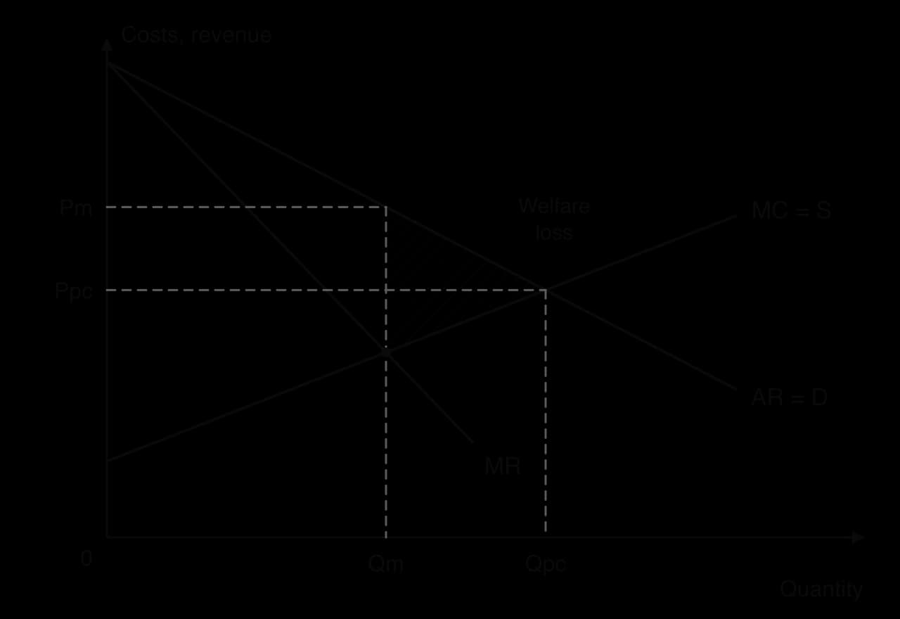
Market with AR = D, MR and MC = S. A competitive market produces Qpc at Ppc where D meets MC. A monopoly produces Qm, where MC = MR, and charges the higher price Pm. The hatched triangle between Qm and Qpc, under D and above MC, is the welfare loss. — The monopolist restricts output to Qm and raises the price to Pm, compared with Qpc and Ppc under perfect competition. The hatched triangle is the welfare loss: units worth more to consumers than they cost are not produced.

At Qm, the price consumers pay (and so the marginal benefit of the last unit) is well above its marginal cost: P > MC. Each unit between Qm and Qpc would be valued by consumers more than it costs to produce, yet the monopolist does not produce it, because doing so would lower the price on all its other units and reduce its profit. Too few resources are allocated to the good, so the outcome is allocatively inefficient, a market failure.

The surplus lost on these units is the welfare loss (deadweight loss), shown by the hatched triangle between the demand curve and the MC curve from Qm to Qpc. Part of the consumer surplus that existed under competition is also transferred to the monopolist as abnormal profit, the rectangle between Pm and Ppc up to Qm. That transfer is not a loss to society as a whole, but it shifts income from consumers to the firm’s owners, which raises a question of equity.

A monopolist is also usually affected by productive inefficiency. It does not have to produce at minimum AC, and with no competitors to put pressure on it, it may let costs rise: managers may tolerate overstaffing, slow decisions or poor service. Waste of this kind is called X-inefficiency.

Natural monopoly

In some industries economies of scale are so large that long-run average cost keeps falling over the whole range of output that the market could buy. The clearest cases are networks: water and sewerage pipes, electricity and gas grids, railway track. Building the network costs a huge amount, but once it exists, supplying an extra household costs very little.

In such a market, competition would raise costs. Two water companies laying two sets of pipes along every street would each serve half the customers at a much higher average cost. One firm is the cheapest way to supply the market, but left alone it would behave like any monopolist.

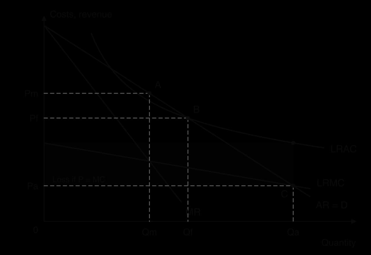
Natural monopoly: LRAC falls over the whole range of demand, with LRMC below it. A: profit maximisation where MC = MR (Qm, Pm). B: price equal to average cost (Qf, Pf). C: price equal to marginal cost (Qa, Pa), below LRAC, with the shaded loss. — LRAC falls over the whole range of demand. Unregulated, the firm produces Qm at Pm (A). Setting P = MC gives the efficient Qa at Pa (C) but a loss, since Pa < LRAC. Setting P = AC (B) gives normal profit at Qf.

The diagram shows why natural monopolies are hard to regulate. Left alone, the firm chooses Qm, where MC = MR, and charges Pm, earning abnormal profit with an allocatively inefficient output. If a regulator forced it to charge a price equal to marginal cost (point C), output would be allocatively efficient, but because LRAC is always falling, marginal cost is always below average cost, and the firm would make a loss on every unit. It would need a subsidy to stay in business.

A common compromise is average cost pricing (point B): the price is set where AR = AC, so the firm covers its costs and earns normal profit, producing more and charging less than an unregulated monopolist, though still less than the allocatively efficient quantity.

In England and Wales, water and sewerage companies are regional natural monopolies, each the only supplier in its area. The regulator, Ofwat, sets limits on the prices they can charge for five years at a time; its most recent review, completed in December 2024, set price limits for 2025–2030.

Sources: Wikipedia, “Ofwat” (accessed 2026).

Oligopoly

Many of the most important markets in modern economies are oligopolies: supermarkets, mobile networks, car manufacturing, commercial aircraft, banking, soft drinks and crude oil. A few large firms account for most of the sales, and high barriers to entry, often economies of scale or brand loyalty, keep the number of firms small.

Interdependence

The defining feature of oligopoly is interdependence. With only a few firms, a price cut by one takes sales from the others, who are likely to respond. Each firm must therefore think about how its rivals will react before it acts, much as a chess player plans several moves ahead. A monopolist or a perfectly competitive firm has no rivals to worry about in this way.

Interdependence creates a basic choice for oligopolists. They can compete, which risks a price war that leaves all of them worse off, or they can cooperate to behave like a single monopolist and share the abnormal profit. Which they choose decides whether the market is a collusive or a non-collusive oligopoly.

Collusive oligopoly

Collusion is an agreement between firms to limit competition between them, for example by fixing prices, limiting output, or dividing up customers or regions. When the firms agree formally to act together as if they were one firm, the arrangement is a cartel.

A cartel tries to reproduce the monopoly outcome. Its members estimate the market demand curve and the combined marginal cost of the industry, choose the total output at which MC = MR, and set the price on the demand curve. Each member then receives an output quota, and together they share the abnormal profit.

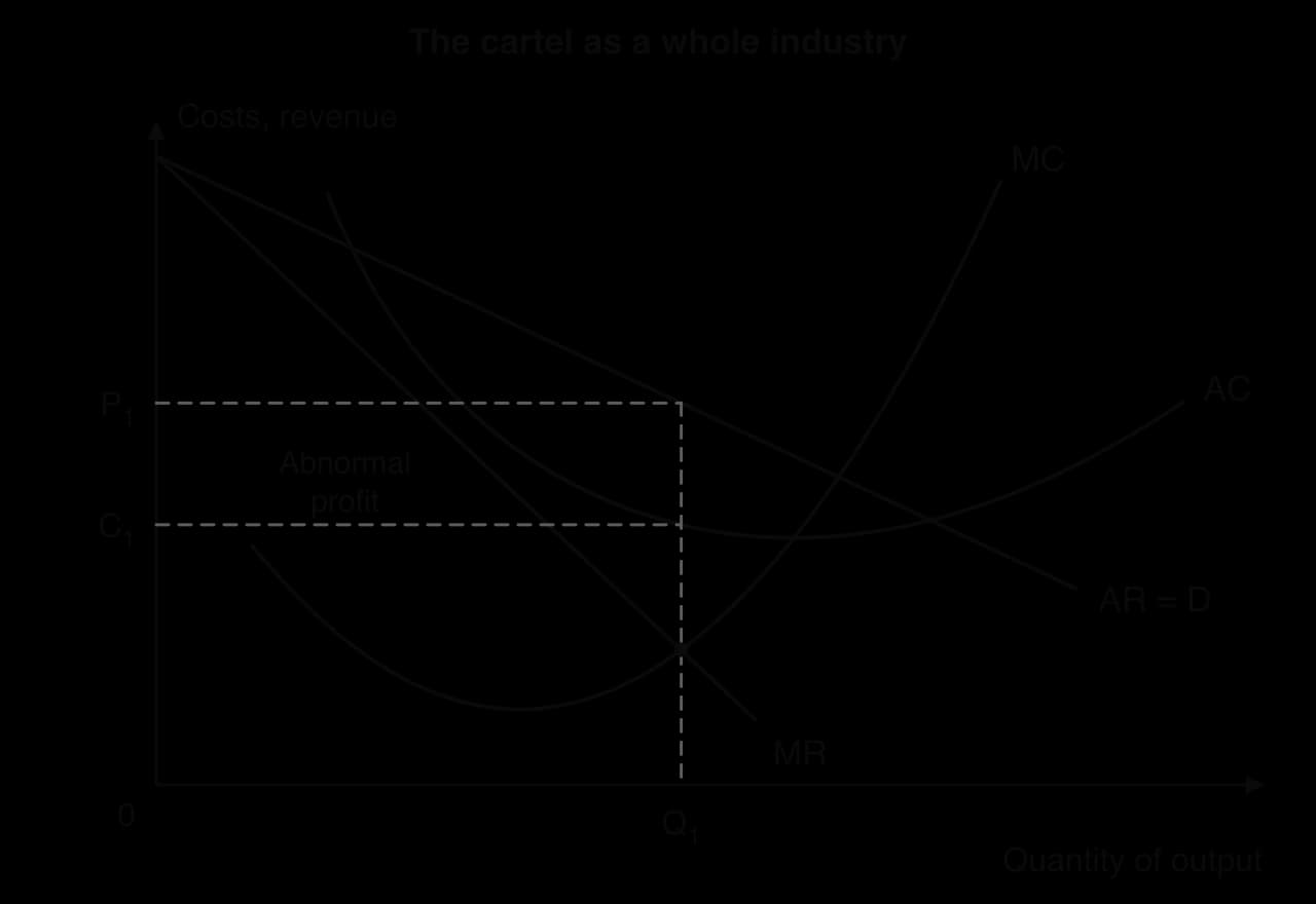
A cartel acting as a monopoly: industry MC, AC, AR = D and MR. Total output is set at Q1 where MC = MR, the price at P1 from the demand curve, average cost is C1, and the abnormal profit rectangle between P1 and C1 is shared among members. — The cartel treats the industry as one monopoly: total output Q₁ where industry MC = MR, price P₁ from demand, and the abnormal profit (P₁ − C₁) × Q₁ shared among members through quotas.

Formal collusion between firms is illegal in most countries, because it harms consumers in exactly the way monopoly does: output is restricted, the price is raised above marginal cost and there is a welfare loss. The Organization of the Petroleum Exporting Countries (OPEC) and its partners, a cartel of governments rather than firms, is the best-known exception, because sovereign states are not subject to national competition law.

Firms can also cooperate without any agreement. In tacit collusion, firms avoid price competition without communicating: for example, one large firm acts as a price leader, and the others follow its price changes. Tacit collusion is harder to prove in court than a written agreement.

The incentive to collude and the incentive to cheat

Every member of a cartel gains from colluding, since together they earn monopoly profit. Each member, however, also has an incentive to cheat. At the cartel price, which is far above marginal cost, any single member could sell extra units secretly, at the cartel price or slightly below it, and add a great deal to its own profit. If only one member cheats, it gains at the expense of the others.

If every member reasons the same way, total output rises, the price falls and the cartel’s abnormal profit disappears. Cartels are therefore unstable. They are more likely to hold together when there are only a few members, when the members have similar costs, when output is easy to monitor, and when cheating can be punished.

Game theory

The conflict between cooperating and cheating can be analysed with game theory, the study of how players make decisions when the outcome for each depends on what the others do. A simple game has two players, each with two possible strategies, and a payoff matrix that shows each player’s outcome for every combination of choices.

Two oil producers, A and B, each decide whether to keep to their agreed quota (cooperate) or to raise output above it (cheat). The payoff matrix gives each producer’s profit in $ billion (hypothetical figures); in each cell, A’s profit comes first.

	B keeps to its quota	B raises output
A keeps to its quota	A: 30, B: 30	A: 10, B: 40
A raises output	A: 40, B: 10	A: 15, B: 15

The game is solved by looking at each player’s best response to each of the other’s choices. A player has a dominant strategy if one strategy gives it a better payoff whatever the other player does.

Using the payoff matrix for producers A and B, (a) identify each producer’s dominant strategy; (b) identify the outcome of the game; (c) explain why both producers would be better off if they could trust each other.

Show the solution

Step 1: A’s best response. If B keeps to its quota, A earns 30 by keeping to its quota and 40 by raising output: raising output is better. If B raises output, A earns 10 by keeping to its quota and 15 by raising output: raising output is better again.

Step 2: (a) dominant strategies. Raising output is better for A whatever B does, so it is A’s dominant strategy. The game is symmetrical, so raising output is B’s dominant strategy too.

Step 3: (b) the outcome. Both producers raise output and each earns $15 billion. Neither can do better by changing its own strategy alone, so neither has a reason to move from this outcome.

Step 4: (c) why trust would pay. If both kept to their quotas, each would earn $30 billion, twice as much. Each producer acting in its own interest produces an outcome that is worse for both. Cooperation would pay, but each fears being the one that keeps to its quota while the other cheats (earning only $10 billion).

The outcome where both players cheat is a Nash equilibrium: given what the other player is doing, neither player can improve its payoff by changing its own choice. Games like this one, where the pursuit of self-interest leaves both players worse off than cooperation would, are known as the prisoner’s dilemma, after a classic example about two suspects who would both do better by staying silent but each has an incentive to confess.

The game explains both why oligopolists want to collude and why collusion breaks down. It also explains why firms try to escape the dilemma: by signing binding agreements (illegal for firms), by building trust over many rounds of the game, or by threatening to punish a cheat with a price war. In a game repeated many times, a strategy of cooperating as long as the rival cooperates can sustain high prices without any formal agreement.

EconplusDal (8 min) on game theory in oligopoly: building a payoff matrix, finding dominant strategies and the Nash equilibrium, and why collusion is unstable.

Non-collusive oligopoly

In a non-collusive oligopoly, firms do not cooperate, but each still takes its rivals’ likely reactions into account. Such markets often show stable prices for long periods. A firm that raises its price fears that rivals will not follow and that it will lose customers; a firm that cuts its price fears that rivals will match the cut, so it gains few customers and all firms end up with lower revenue.

When this stability breaks down, the result can be a price war: a series of price cuts as each firm tries to win market share from the others. Price wars benefit consumers in the short run but can drive the weakest firms out of the market, leaving it more concentrated afterwards.

Reliance Jio’s entry into the Indian mobile market is a clear case. Jio launched its 4G network publicly on 5 September 2016 offering free data and calls until 31 March 2017, and reached 100 million subscribers by February 2017. The launch set off a fierce price war, with sharply falling call and data tariffs. Many smaller operators left: Telenor India was taken over by Bharti Airtel in 2018, Aircel filed for bankruptcy in March 2018, and Vodafone India and Idea Cellular merged in August 2018 to form Vodafone Idea. By July 2026 three networks, Jio (39.3%), Airtel (38.0%) and Vodafone Idea (15.5%), held about 93% of wireless subscribers.

Sources: Wikipedia, “Jio”, “Vodafone Idea” and “Telecommunications in India”, citing TRAI subscriber data for July 2026 (accessed 2026).

Price and non-price competition

Because price competition is risky, oligopolists often prefer non-price competition. Firms compete through advertising, brand names, product design, quality, packaging, loyalty schemes, after-sales service and the range of products they offer. These methods are harder for rivals to copy instantly than a price cut, and they build brand loyalty, which makes demand for the firm’s product less price elastic and raises a barrier to new entrants.

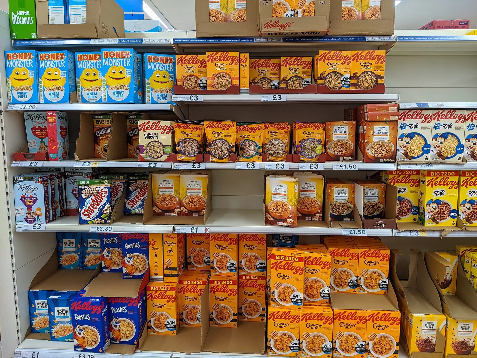
Supermarket breakfast cereal shelves filled mostly with Kellogg's brands (Crunchy Nut, Coco Pops, Frosties) alongside a few Nestlé, Honey Monster and Tesco own-label boxes, in many flavours and pack sizes. — Breakfast cereals are an oligopoly: a few producers fill the shelves with many brands, flavours and pack sizes, competing for shelf space and loyalty more than on price. Photo: Vauxford, CC BY-SA 4.0, via Wikimedia Commons.

Brand proliferation, selling many brands of what is essentially the same product, is a form of non-price competition that also deters entry: when a few producers already fill a supermarket’s shelves with dozens of brands, there is little room left for a new entrant.

Measuring market concentration

Whether a market is an oligopoly is judged by how much of it the largest firms control. A concentration ratio adds up the market shares of the largest firms. The four-firm concentration ratio (CR4) is the combined share of the four largest firms; as a rough guide, a CR4 above about 50% is often taken to indicate an oligopoly.

Grocery retailer (Great Britain)	Market share, 12 weeks to 20 April 2025 (%)
Tesco	27.8
Sainsbury’s	15.3
Asda	12.3
Aldi	11.0
Lidl	8.0
Waitrose	4.5
Ocado	1.9

Sources: Kantar grocery market share data, reported by Grocery Gazette, 29 April 2025. The table lists only the retailers whose shares the report gives; Morrisons, Co-op, M&S and Iceland are not shown.

Concentration ratios are easy to calculate and to compare over time, but they have limits. They depend on how the market is defined (all groceries, or only online groceries; one country, or the world), they say nothing about how market shares are distributed among the top firms, and a high ratio does not prove that firms behave uncompetitively, since a few large firms may still compete fiercely.

Oligopoly and allocative inefficiency

Oligopolies usually fail to achieve allocative efficiency. A collusive oligopoly behaves like a monopoly, restricting output so that P > MC and creating a welfare loss. Even without collusion, each firm has a downward-sloping demand curve, sets price above marginal cost and earns abnormal profit protected by barriers to entry. On the other hand, oligopolies may achieve large economies of scale and spend heavily on research and development, and intense non-price competition can bring new products and better quality.

Monopolistic competition

Monopolistic competition combines features of perfect competition and monopoly. As in perfect competition, there are many firms and entry and exit are free. As in monopoly, each firm sells a product that is slightly different from all the others, so it faces a downward-sloping demand curve and is a price maker.

Coffee shops, restaurants, hairdressers, clothing boutiques and plumbers are typical examples. A hair salon can charge slightly more than its rivals because some customers prefer its stylists, its location or its atmosphere, but if it raises its price too far, many customers will switch to one of the many alternatives nearby.

The short run

In the short run a monopolistically competitive firm behaves like a small monopolist. It produces where MC = MR and charges the price on its demand curve. Depending on demand and costs, it may earn abnormal profit or make a loss.

Two monopolistically competitive firm panels with AR = D and MR. Left: MC = MR at Q1, price P1 above average cost C1, abnormal profit shaded. Right: a flatter AR; MC = MR at Q1 on the rising part of MC, price P1 below average cost C1, loss shaded. — In the short run the firm produces where MC = MR and may earn abnormal profit (left, P₁ > C₁) or make a loss (right, P₁ < C₁), just like a monopolist.

The long run: normal profit and excess capacity

Without barriers to entry, the short run does not last. Abnormal profit attracts new firms with similar products. Each existing firm loses some customers to the newcomers, so the demand curve it faces shifts to the left (and may become more elastic, since there are now more close substitutes). This continues until the demand curve just touches the AC curve at the output where MC = MR: the firm earns only normal profit. If firms are making losses, some leave, and the demand for each remaining firm rises until normal profit is restored.

Monopolistic competition in the long run: AR = D is tangent to AC at T, at output Q1 where MC = MR, so price P1 equals average cost (normal profit). Q1 lies left of Qmin, the output at minimum AC; the gap is labelled excess capacity. — In long-run equilibrium AR is tangent to AC at T: price P₁ equals average cost, so the firm earns normal profit. Its output Q₁ is below Qmin, where AC is lowest, leaving excess capacity.

The tangency point is to the left of the minimum of the AC curve, because the demand curve slopes down and can only touch the U-shaped AC curve where AC is also falling. The firm therefore produces less than the output at which its average cost would be lowest. The difference is called excess capacity: each firm could produce more at a lower cost per unit, but demand for its particular product is not large enough.

Excess capacity shows up as cafés with empty tables for much of the day and hairdressers waiting for customers between appointments. Many small firms each produce at a higher average cost than fewer, larger ones would.

Efficiency in monopolistic competition

Even in long-run equilibrium, price is above marginal cost (at Q₁, AR lies above MC), so monopolistic competition is allocatively inefficient. Output is below minimum AC, so it is productively inefficient as well.

The inefficiency is much smaller than under monopoly. Because there are many close substitutes, each firm’s demand curve is much more elastic than a monopolist’s, so the gap between price and marginal cost is small. Free entry also removes abnormal profit in the long run, so consumers do not pay for a lasting transfer of surplus to producers.

Two panels with the same cost curves. Monopoly: steep AR, price P1 far above MC and average cost C1, abnormal profit shaded. Monopolistic competition: flatter, more elastic AR tangent to AC at Q1, price P1 equal to average cost, closer to MC. — With the same costs, the monopolist’s steep AR lets it set P₁ far above MC and keep abnormal profit. The monopolistic competitor’s flatter, more elastic AR keeps P₁ close to MC, with only normal profit in the long run.

Monopolistic competition also gives consumers something perfect competition cannot: variety. Many consumers are willing to pay a slightly higher price to have a choice of cafés, restaurants and styles. The higher average cost from excess capacity can be seen as the price of this variety, and whether it is worth paying is partly a value judgement.

Comparing the four market structures

Outcome	Perfect competition	Monopolistic competition	Oligopoly	Monopoly
Long-run profit	Normal	Normal	Often abnormal	Usually abnormal
Price compared with MC	P = MC	P > MC, small gap	P > MC	P > MC, large gap
Allocative efficiency	Yes	No (small welfare loss)	No	No (largest welfare loss)
Productive efficiency (long run)	Yes, at minimum AC	No: excess capacity	Not necessarily	Not necessarily
Economies of scale	None	Few	Often large	Often large
Funds for R&D	None	Little	Large	Large
Product variety	None	High	Varies; often many brands	One product line

Advantages of large firms with significant market power

The analysis so far suggests that market power always harms consumers. That conclusion depends on an assumption hidden in the comparison of monopoly with perfect competition: that costs are the same in both. In many industries they are not, and large firms with market power can bring real benefits.

Economies of scale

A large firm can often produce at a much lower average cost than many small firms. If its costs are low enough, even a profit-maximising firm with market power may charge a lower price and produce more than a competitive industry of small, high-cost firms. Natural monopolies are the extreme case: competition would require wasteful duplication of networks, so one firm, regulated, supplies the market most cheaply.

Economies of scale also help firms compete in world markets. Building commercial aircraft, designing advanced microchips or developing new medicines requires such large fixed costs that only very large firms can spread them over enough output to keep average cost down.

Abnormal profit, research and development, and innovation

Abnormal profit, protected by barriers to entry, gives large firms both the funds and the incentive for research and development (R&D). A firm in perfect competition earns only normal profit, and any new idea is quickly copied. A firm with market power can finance expensive, risky research from its profits and, if the research succeeds, keep the reward for long enough to make the risk worthwhile. Patents exist to create exactly this temporary market power.

Nvidia, a designer of the chips used to train artificial intelligence models, shows the link between profit and R&D. In its 2025 financial year, which ended in January 2025, it reported revenue of $130.5 billion, a gross margin of 75% and net income of $72.9 billion, and it spent $12.9 billion on research and development. Revenue from its data centre business, where its AI chips are sold, had risen by 142% in a year to $115.2 billion.

Sources: Nvidia, financial results for the fourth quarter and fiscal 2025 (February 2025).

Innovation of this kind brings gains that a static comparison of welfare triangles misses: new products, better quality and lower costs over time. Some economists argue that these long-run gains outweigh the short-run welfare loss from market power, and that the prospect of temporary monopoly profit is what drives innovation in a market economy.

Other possible advantages

Stability: large, profitable firms can absorb shocks, keep investing through a downturn and offer more secure employment.
Standards and compatibility: one dominant network or standard (a payment system, an operating system) can be more useful to consumers than several incompatible ones.
Cross-subsidy: a firm with market power, such as a postal service or a national railway, can use profits on busy routes to keep services running in remote areas.

Risks of markets dominated by a few very large firms

When one or a few very large firms dominate a market, the risks fall on output, price and consumer choice, and spread further to the rest of the economy.

Higher prices and lower output: firms restrict output to the point where MC = MR, so price is above marginal cost and there is a welfare loss. Consumers pay more and buy less than in a competitive market.
Less consumer choice: with fewer firms, consumers have fewer alternatives, and a dominant firm can decide which products reach the market. When a dominant search engine or platform favours its own services, rivals’ products may never be seen.
Complacency and productive inefficiency: protected from competition, firms may let costs rise and quality fall, and may have less pressure to innovate than firms fighting for customers.
Barriers that block new ideas: dominant firms can buy up or squeeze out small, innovative rivals, so the innovation advantage of large firms may be outweighed by the innovation they prevent.
Equity: abnormal profit transfers income from consumers to the owners of firms, who are on average richer, adding to inequality.
Power over suppliers, workers and governments: very large firms can push down the prices they pay suppliers and the wages they pay workers where they are the main buyer, and can use their size to lobby governments for favourable rules.

Weighing the advantages against the risks

Whether a market dominated by large firms is good or bad for society depends on the circumstances, and a judgment needs to weigh several factors.

What the judgment depends on	Market power is less harmful when…	Market power is more harmful when…
Size of economies of scale	they are large, so a few firms produce much more cheaply	they are small, so higher prices bring no cost saving
Use of abnormal profit	it is reinvested in R&D that brings new products and lower costs	it is paid out to owners while quality and investment stagnate
Ease of entry	new firms (or imports) can enter if prices rise, which limits the dominant firm’s behaviour	barriers are high and permanent
Time period	market power is temporary, like a patent that expires	dominance lasts for decades
Regulation	a strong, well-informed regulator controls prices and quality	regulators are weak, slow or influenced by the firms
Type of product	close substitutes exist	the product is essential (water, energy, medicines) and demand is price inelastic

The effect of large firms therefore depends on the market. Market power is most likely to harm society when it is protected by high and lasting barriers, when it is used to raise prices for essential goods, and when it does not come with lower costs or innovation. These are the cases where government responses are most justified.

Government responses to the abuse of market power

Governments respond to market power in three main ways: legislation and regulation, government ownership, and fines. Each is a form of intervention that tries to bring the outcome closer to the allocatively efficient one without losing the benefits that large firms can bring.

Legislation and regulation

Most countries have competition laws (also called antitrust or anti-monopoly regulation) enforced by a competition authority, such as the European Commission in the EU or the Competition Commission of India. These laws typically do three things.

Ban cartels: agreements between firms to fix prices, limit output or share out markets are illegal.
Ban the abuse of a dominant position: a dominant firm may not, for example, charge excessive prices, cut prices below cost to drive out rivals, force customers to buy one product in order to get another, or favour its own services over rivals’ on a platform it controls.
Control mergers: large mergers must be approved in advance, and the authority can block a merger, or approve it only with conditions, if it would reduce competition substantially. In extreme cases, a dominant firm can be ordered to break itself up.

For natural monopolies, where competition is not practical, governments regulate prices and quality directly. A price cap limits how much the regulated firm may raise its prices, often to inflation minus an amount for expected efficiency gains, for a fixed period such as five years. Because the firm keeps any extra profit from cutting costs below what the regulator expected, a price cap gives it an incentive to become more efficient. Regulators can also require the owner of a network to let competitors use it on fair terms, which opens up competition in the services provided over the network.

Evaluation

Strengths: legislation deters anti-competitive behaviour across the whole economy; merger control can prevent harmful market power before it arises; price regulation protects consumers of essential services while keeping the cost advantage of a single network.
Limitations: regulators have less information than the firms about costs and demand, so price caps may be set too high (leaving abnormal profit) or too low (discouraging investment); cases take years, and markets, especially digital ones, change faster than the law; regulators may be influenced by the firms they regulate (regulatory capture); and very large multinational firms can be hard for any single country to control.

Government ownership

A government can take a natural monopoly or a strategic industry into public ownership and run it as a state-owned enterprise, setting prices with the public interest in mind rather than profit. In principle, a state-owned firm can charge a price closer to marginal cost, accept lower profits (or a loss covered by taxes), and provide services to remote or low-income areas that a private monopolist would neglect.

Eskom, South Africa’s state-owned electricity utility, generates about 95% of the electricity used in the country, a natural monopoly in public hands. It has also shown the risks of government ownership. Rolling power cuts (“load shedding”) have been used since 2008, reaching up to 12 hours a day in the winter of 2023; by February 2023 Eskom’s debt stood at R423 billion, and the government announced debt relief worth R254 billion.

Sources: Wikipedia, “Eskom” (accessed 2026).

Evaluation

Strengths: prices can be set for social goals such as affordability and universal service; profits stay with the public; essential networks can be planned for the long term.
Limitations: without the profit motive or competition, state-owned firms may become productively inefficient; decisions may be driven by politics, such as keeping prices low before an election and underinvesting; losses fall on taxpayers, with an opportunity cost in other public spending. These problems are one reason many governments chose privatisation of state-owned utilities from the 1980s onwards, combined with regulation.

Fines

Competition authorities can fine firms that break competition law. Two cases show fines used against both forms of market power.

Collusion: in July 2016 the European Commission imposed a then-record fine of €2.93 billion on truck makers that had run a 14-year cartel on truck prices and on passing on to customers the cost of meeting emission standards. The five members, MAN, Volvo/Renault, Daimler, Iveco and DAF, together made about 9 out of every 10 medium and heavy trucks produced in Europe. MAN was not fined because it had revealed the cartel to the Commission.
Abuse of dominance: in June 2017 the Commission fined Google €2.42 billion for abusing its dominance in search by promoting its own comparison shopping service in its search results and demoting rivals’. The EU’s General Court upheld the fine in 2021, and the Court of Justice confirmed it in September 2024.

Sources: European Commission press releases IP/16/2582 (2016) and IP/17/1784 (2017); Wikipedia, article on the European Union’s Google cases (accessed 2026).

The MAN case shows how leniency programmes use the logic of game theory against cartels. The first member to confess and give evidence escapes the fine, so each member has an incentive to report the cartel before another does. The cartel members face a new prisoner’s dilemma, in which betraying the others becomes the dominant strategy.

Evaluation

Strengths: fines punish past abuse and deter future abuse; they raise revenue rather than costing the government money; combined with leniency, they make cartels harder to sustain.
Limitations: to deter, the expected fine (the fine multiplied by the probability of being caught) must exceed the expected gain from the abuse, and many cartels are never detected; fines arrive years after the harm, which has already fallen on consumers; a fine alone does not restore competition unless the behaviour also changes; and a firm may pass the cost of a fine on to consumers through higher prices.

Key concepts at work

Key concept	How it applies to market power
Efficiency	Market power causes allocative inefficiency (P > MC) and often productive inefficiency; economies of scale and R&D can raise efficiency over time.
Equity	Abnormal profit transfers surplus from consumers to the owners of firms.
Interdependence	Oligopolists must take their rivals’ reactions into account; game theory models the consequences.
Intervention	Competition law, price regulation, public ownership and fines aim to limit the abuse of market power.
Change	Innovation, new entrants and new technology can erode market power, as when new rivals enter a market or a patent expires.

Case study: OPEC+ in 2020, from price war to collusion

OPEC+ is the group formed in late 2016 by the members of OPEC and other oil-exporting countries, led by Russia, to coordinate cuts in crude oil output. It is a cartel of governments: by agreeing on production quotas, its members aim to keep the price of oil above the level that competition between them would produce. Its experience in 2020 shows every part of oligopoly theory at work: collusion, the incentive to cheat, a price war and a return to cooperation.

In early 2020 the spread of COVID-19 was cutting the world’s demand for oil. At a meeting on 5 March 2020, OPEC proposed a further cut in output of 1.5 million barrels per day (mb/d). On 6 March Russia rejected it, and the existing agreement on cuts was due to expire at the end of March. Saudi Arabia, the largest OPEC producer, responded by offering discounts of $6–8 a barrel to its customers and announcing that it would raise its output from about 9.7 mb/d to 12.3 mb/d, so the cartel collapsed into a price war.

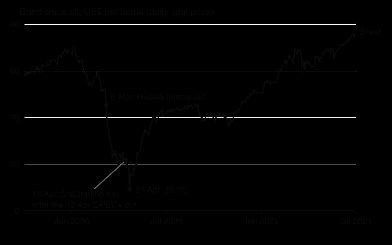
Line chart of the daily Brent crude oil price from October 2019 to June 2021. About –70 until January 2020, falling to .60 on 6 March, .12 on 21 April 2020, then recovering to about by mid-2020, at the end of 2020 and by June 2021. — Brent fell from $51.29 on 5 March 2020 to $35.33 on 9 March after the OPEC+ talks failed, and reached $9.12 on 21 April. After the April output cut it recovered to $51 by the end of 2020. Source: FRED, Federal Reserve Bank of St Louis, series DCOILBRENTEU (2026).

The price of Brent crude, the main international benchmark, fell by 31% between 5 and 9 March, across Russia’s refusal and Saudi Arabia’s response, from $51.29 a barrel on 5 March to $35.33 on 9 March. With demand collapsing as countries locked down and producers pumping more, storage began to run out. On 20 April the US benchmark, West Texas Intermediate, closed at −$36.98 a barrel: sellers were paying buyers to take oil they had nowhere to store. Brent reached its low of $9.12 on 21 April.

The episode follows the payoff matrix of a prisoner’s dilemma closely. Each producer gained from the cartel’s high price, but each also had an incentive to produce more than its share. Russia was unwilling to cut its own output while the United States, outside the cartel, kept producing shale oil and gaining market share. Saudi Arabia’s response, flooding the market, was a threat made real: a punishment that hurt every producer, including itself, and that made the gains from cooperation obvious to all.

Cooperation returned within weeks. On 12 April 2020 the 10th (Extraordinary) OPEC and non-OPEC Ministerial Meeting agreed a cut equal to about a tenth of world oil output. Members would reduce production by 9.7 mb/d from 1 May for two months, by 7.7 mb/d from July to December 2020, and by 5.8 mb/d from January 2021 to April 2022, measured from their October 2018 output (with a baseline of 11.0 mb/d for both Saudi Arabia and Russia). The schedule was adjusted at later meetings, starting with an extension of the deepest cut into July 2020.

The quotas restricted industry output in exactly the way the collusive oligopoly diagram predicts, and as demand recovered the price rose: Brent was $41.64 at the end of June 2020, $51.22 at the end of 2020 and $76.94 at the end of June 2021.

Date	Event	Brent price (US$ per barrel)
5 March 2020	OPEC proposes a further 1.5 mb/d cut	51.29
6 March 2020	Russia rejects the cut	45.60
9 March 2020	First trading day after Saudi Arabia’s discounts	35.33
21 April 2020	Low point, with storage nearly full	9.12
30 June 2020	9.7 mb/d cut in force	41.64
31 December 2020	Smaller cuts in force; demand recovering	51.22
30 June 2021	Agreement still in force; it ran to April 2022	76.94

The case also shows the limits of the theory and of the cartel. Most of the price collapse was caused by the fall in demand during the pandemic, which no cartel could prevent, so the price war is only part of the explanation. The cartel controls only part of world supply, and producers outside it, such as the United States, benefit from its cuts without bearing their cost. Compliance with quotas has to be monitored and enforced among sovereign states, which no court can do. The cartel’s success is also a cost to others: higher oil prices transfer income from consumers and oil-importing countries to producers, an issue of equity as well as efficiency.

Sources: FRED, Federal Reserve Bank of St Louis, series DCOILBRENTEU and DCOILWTICO (accessed 2026); OPEC, press release on the 10th (Extraordinary) OPEC and non-OPEC Ministerial Meeting (12 April 2020); Wikipedia, “2020 Russia–Saudi Arabia oil price war” and “OPEC+” (accessed 2026).

Exam practice

Market power is HL material, so questions on it appear in HL Paper 1 (extended response) and HL Paper 3 (policy paper), but not in Paper 2, which is the same for SL and HL and contains no HL material. Paper 3 often uses cost and revenue tables, payoff matrices and concentration ratios for short calculations, and Paper 1 questions usually ask for a diagram of one market structure followed by an evaluation of market power or of government policy.

Paper 1, part (a) [10 marks]: Using an appropriate diagram, explain why a monopoly is likely to be allocatively inefficient.

Show an answer plan

Define the terms. Monopoly: a single firm, or dominant firm, with no close substitutes and high barriers to entry. Allocative efficiency: resources produce the goods society values most, where P = MC (MB = MC) and social surplus is maximised.

Draw the diagram. Monopoly compared with perfect competition: D = AR, MR, MC = S. Mark Qm and Pm where MC = MR, and Qpc and Ppc where D meets MC. Hatch the welfare loss triangle between Qm and Qpc.

Explain the mechanism. The monopolist maximises profit where MC = MR. Because it must cut its price on all units to sell one more, MR is below AR, so at Qm the price Pm is above MC. Units between Qm and Qpc are valued by consumers above their cost but are not produced: too few resources go to the good.

Explain the result. Social surplus is not maximised; the hatched triangle is the welfare loss. Part of the consumer surplus is transferred to the monopolist as abnormal profit, which barriers to entry protect in the long run. Refer to each point on the diagram as you explain it.

Part (b) of the same question usually widens the theory of part (a) into an evaluation of policy or of market power in general, and needs developed real-world examples.

Paper 1, part (b) [15 marks]: Using real-world examples, evaluate the view that governments should always act to reduce the market power of large firms.

Show an answer plan

Theory (briefly, linked to the diagram in (a)). Market power lets firms set P > MC, restrict output and earn lasting abnormal profit: allocative inefficiency, welfare loss and a transfer from consumers to producers. Collusive oligopoly behaves like a monopoly.

Arguments for acting. Cartels raise prices with no offsetting benefit (EU trucks cartel, 14 years, €2.93 billion fine, 2016). Dominant platforms can restrict consumer choice and shut out rivals (Google Shopping, €2.42 billion, upheld by the EU Court of Justice in 2024). Essential goods with inelastic demand leave consumers exposed.

Arguments against “always”. Economies of scale can make one firm the cheapest supplier (natural monopolies such as water networks, where regulation, not break-up, is the answer). Abnormal profit can fund R&D (Nvidia spent $12.9 billion on R&D in its 2025 financial year; patents deliberately create temporary monopoly to reward innovation). Intervention has costs: regulators lack information, cases are slow, and state ownership can be inefficient (Eskom’s load shedding and debt).

Judgment. The word “always” is too strong. Governments should act firmly against collusion and abuse of dominance, where there is harm with no benefit, and regulate natural monopolies; but large size and high market share alone, when they bring lower costs and innovation and when entry remains possible, do not justify intervention. The right response depends on the source of the power, the barriers to entry and the type of product.

Paper 3-style items

The following short items use the style of HL Paper 3, part (a). Work them before opening the answers.

Define the term natural monopoly. [2]
A firm produces 200 units at a total cost of $3,000 and sells them at $18 each. Calculate its average cost and its total abnormal profit. [2]
When the firm in item 2 raises output from 200 to 220 units, its total cost rises to $3,330 and its price must fall to $17.50. Calculate the marginal cost and the marginal revenue of these extra units, and state whether the increase in output raises profit. [3]
The five largest firms in a market have shares of 31%, 22%, 14%, 9% and 7%. Calculate the four-firm concentration ratio. [1]
Draw a diagram of a natural monopoly showing the output and price if it is regulated so that price equals average cost. [3]

Show the answers

1. A market in which long-run average cost falls over the whole range of market demand [1], so one firm can supply the market at a lower average cost than two or more firms could [1].

2. AC = $3,000 ÷ 200 = $15. Abnormal profit = (AR − AC) × Q = ($18 − $15) × 200 = $600.

3. MC = ΔTC ÷ ΔQ = ($3,330 − $3,000) ÷ 20 = $16.50 per unit. TR rises from 200 × $18 = $3,600 to 220 × $17.50 = $3,850, so MR = $250 ÷ 20 = $12.50 per unit. Since MR < MC, the extra output reduces profit (by $330 − $250 = $80).

4. CR4 = 31 + 22 + 14 + 9 = 76%.

5. Axes labelled “Costs, revenue” and “Quantity”; LRAC falling throughout, with LRMC below it; AR = D cutting LRAC on its falling part; the regulated output where AR = AC marked on the quantity axis and the price on the vertical axis.

Paper 3, part (b) [10 marks]: A country’s electricity grid is owned by a single private company that earns large abnormal profits, while households complain about high prices and frequent power cuts. Using the information and your knowledge of economics, recommend a policy the government could introduce to deal with this market power.

Show an answer plan

Choose one policy and state it clearly. For example: price-cap regulation by an independent regulator for five-year periods, with quality targets on reliability and penalties for power cuts.

Explain the theory. The grid is a natural monopoly (LRAC falling over the whole market), so competition would duplicate costly networks. Unregulated, the firm sets MC = MR, charging Pm with output below the efficient level; a cap moves the price towards average cost (normal profit), raising output and cutting the welfare loss. Draw the natural monopoly diagram.

Use the case’s information. Refer to the abnormal profits as evidence that price is above AC, and to the power cuts as evidence that quality, not just price, needs regulating.

Evaluate. The regulator lacks information on true costs; a cap set too low may cut investment and worsen power cuts; regulatory capture is a risk. Compare briefly with public ownership (lower prices possible but risk of inefficiency and political interference, as Eskom shows) and justify why regulation is preferred here. End with a clear recommendation.

Summary

Markets range from perfect competition (no market power) through monopolistic competition and oligopoly to monopoly; barriers to entry decide whether abnormal profit can last.
Every firm maximises profit where MC = MR and charges the price on its AR curve; AR > AC gives abnormal profit, AR = AC normal profit and AR < AC a loss.
A perfectly competitive firm is a price taker (P = D = AR = MR); entry and exit drive it to normal profit at minimum AC in the long run, with P = MC, so the market is allocatively efficient.
A monopolist restricts output and sets P > MC, causing a welfare loss compared with perfect competition; a natural monopoly has falling LRAC over the whole market and is usually regulated or publicly owned.
Oligopolists are interdependent: collusion reproduces monopoly, but each member has an incentive to cheat, as the prisoner’s dilemma shows; concentration ratios measure how far a market is dominated by a few firms.
Monopolistic competition has normal profit and excess capacity in the long run, with a more elastic demand curve, less inefficiency than monopoly and more product variety.
Large firms can bring economies of scale and R&D, but risk higher prices, lower output and less choice; governments respond with legislation and regulation, government ownership and fines.

Self-check

To do:
I can describe the four market structures and explain how barriers to entry separate them.
To do:
I can calculate TC, AC, AVC, MC, TR, AR, MR and profit from data.
To do:
I can explain why profit is maximised where MC = MR and show abnormal profit, normal profit and losses on a diagram.
To do:
I can draw a perfectly competitive firm as a price taker, in the short run and the long run, and explain the shut-down price.
To do:
I can explain allocative efficiency (P = MC) and show it on a competitive market diagram.
To do:
I can draw and explain the welfare loss of monopoly compared with perfect competition, and a natural monopoly diagram.
To do:
I can use a payoff matrix to find dominant strategies and explain why cartels are unstable.
To do:
I can calculate a concentration ratio and comment on what it shows.
To do:
I can draw monopolistic competition in the short run and the long run, and compare its demand curve with a monopoly’s.
To do:
I can evaluate large firms and government responses to market power using real examples.

Questions on 2.11

104 exam-style questions on this subtopic, written in the style of the IB papers. The first has its markscheme open. Counted on 20 October 2026

Question 1 · ECON-000038 marks

A monopoly faces the demand curve $P = 100 - 2Q$ and has constant marginal cost of $20 per unit.

Output (Q)	10	15	20	25
Price ($)	80	70	60	50
Total revenue ($)	800	1050	1200	1250

(a)
Calculate the profit-maximising level of output.
2 marks
Markscheme (a)
$MR = 100 - 4Q = 20$ 1
$Q = 20$ 1
(b)
Calculate the price the monopolist charges.
2 marks
Markscheme (b)
$P = 100 - 2(20)$ 1
$P = \$60$ 1
(c)
Explain why this outcome is allocatively inefficient.
4 marks
Markscheme (c)
$P > MC$ at the chosen output ($60 > $20). 2
Output is restricted below the level where $P = MC$ (Q = 40), creating a welfare loss. 2

Question 2 · ECON-0002925 marks

Efficiency is one of the central concepts in economics.

(a)
Using a production possibilities curve (PPC), explain why an economy producing on its PPC may be productively efficient but not allocatively efficient.
10 marks
(b)
Using real-world examples, evaluate the view that firms with significant market power always use resources inefficiently.
15 marks

Answer it, then compare with the markscheme.Check this one with a free account

Question 3 · ECON-0017925 marks

In some markets a small number of large firms compete intensively through advertising rather than price.

(a)
Explain why a successful advertising campaign by one firm may reduce the demand for a rival firm's product.
10 marks
(b)
Using real-world examples, evaluate the view that significant market power held by large firms is always undesirable.
15 marks

Answer it, then compare with the markscheme.Check this one with a free account

Key terms introduced here

Carry on with 2.11 in Augment

Key terms introduced here

Carry on with 2.11 in Augment

Notes on 2.11 Market failure: market power

Learning objectives

Introduction

Market structures

Perfect competition

Monopoly

Imperfect competition: oligopoly and monopolistic competition

Where barriers to entry come from

Costs of production

Total, fixed and variable costs

Average and marginal costs

The shapes of the short-run cost curves

Long-run costs: economies and diseconomies of scale

Revenue

Revenue curves of a price taker

Revenue curves of a price maker

Profit maximisation

Normal profit, abnormal profit and losses

Why profit is maximised where MC = MR

Reading profit from a diagram

Degrees of market power

Perfect competition

The assumptions of the model

The firm as a price taker

Short-run profit maximisation

Abnormal profit in the short run

Losses in the short run and the shut-down price

The long run: entry, exit and normal profit

Allocative efficiency in perfect competition

Evaluating perfect competition as a benchmark

Monopoly

Sources of monopoly power

Profit maximisation by a monopolist

Allocative inefficiency and welfare loss

Natural monopoly

Oligopoly

Interdependence

Collusive oligopoly

The incentive to collude and the incentive to cheat

Game theory

Non-collusive oligopoly

Price and non-price competition

Measuring market concentration

Oligopoly and allocative inefficiency

Monopolistic competition

The short run

The long run: normal profit and excess capacity

Efficiency in monopolistic competition

Comparing the four market structures

Advantages of large firms with significant market power

Economies of scale

Abnormal profit, research and development, and innovation

Other possible advantages

Risks of markets dominated by a few very large firms

Weighing the advantages against the risks

Government responses to the abuse of market power

Legislation and regulation

Evaluation

Government ownership

Evaluation

Fines

Evaluation

Key concepts at work

Case study: OPEC+ in 2020, from price war to collusion

Exam practice

Paper 3-style items

Summary

Self-check

Questions on 2.11

Markscheme (a)

Markscheme (b)

Markscheme (c)

Try a quick-fire question

Flashcards for 2.11