 YouTube
Explain how governments raise revenue and spend, use AD/AS diagrams to analyse expansionary and contractionary fiscal policy in Keynesian and new classical views, calculate the multiplier (HL) and evaluate fiscal policy.
Each is in the Economics glossary, with every other term in the subject.
Features of the tax and benefit system, such as progressive income taxes and unemployment benefits, that automatically dampen rises and falls in aggregate demand without any new government decision.
A government budget in which government revenue equals government spending over the year, so there is neither a deficit nor a surplus.
The amount by which government revenue exceeds government spending in a given year.
Government spending on investment in long-lasting productive assets, such as roads, railways, schools and hospitals, that add to the economy’s infrastructure.
A cut in government spending, an increase in taxes, or both, intended to reduce aggregate demand or a budget deficit; when aimed mainly at the deficit it is often called austerity.
A demand-side policy that acts against the business cycle, raising aggregate demand in a downturn and reducing it in a boom, to reduce fluctuations in output.
The fall in private sector spending, especially investment, that occurs when increased government borrowing raises interest rates, reducing the effect of expansionary fiscal policy on aggregate demand.
Describe the sources of government revenue and the types of government spending.
Explain the goals of fiscal policy and how changes in government spending and taxation affect aggregate demand.
Draw and explain AD/AS diagrams showing expansionary and contractionary fiscal policy in the Keynesian and monetarist/new classical views.
Explain the Keynesian multiplier and how leakages determine its size (HL).
Calculate the value of the multiplier and the effect on real GDP of a change in an injection (HL).
Draw and explain a diagram showing crowding out (HL).
Explain how progressive taxes and unemployment benefits act as automatic stabilisers (HL).
Evaluate the effectiveness of fiscal policy in achieving economic growth, low unemployment and low and stable inflation.
Fiscal policy is the use of government spending and taxation to influence the level of economic activity. Together with monetary policy it forms demand management: policy that changes aggregate demand (AD) to smooth the business cycle and to steer the economy towards low unemployment, low and stable inflation and steady growth.
Every government budget is an intervention in the economy and a set of choices about scarcity: money spent on hospitals cannot also be spent on roads, and every tax affects who carries the cost. Fiscal policy therefore also raises questions of equity (who pays and who benefits) and of sustainability, because borrowing today must be serviced by taxpayers in the future.
207 exam-style questions on this subtopic, written in the style of the IB papers. The first has its markscheme open. Counted on
The circular flow of income model shows how money flows between decision-makers in an economy.
Using the circular flow of income model, explain how changes in leakages and injections affect the level of national income.
10 marks
Answers may include:
Terminology: definitions of circular flow of income, leakages (withdrawals: saving, taxes, imports), injections (investment, government spending, exports), national income.
Explanation: households receive factor incomes from firms and spend on goods and services; part of income is withdrawn from the flow through saving, taxes and spending on imports; spending is added to the flow by firms' investment, government spending and foreign purchases of exports; if injections exceed leakages, the flow of income and output grows; if leakages exceed injections, the flow shrinks; national income is in equilibrium when total leakages equal total injections (S + T + M = I + G + X).
Diagram: a circular flow diagram with households and firms, flows of factor services, factor incomes, goods and services and consumption expenditure; the financial sector, government and foreign sector shown with S, T and M as leakages and I, G and X as injections.
A maximum of [6] should be awarded if only leakages or only injections are explained.
Markbands (best fit)
Level | Marks | Descriptor |
|---|---|---|
One of 51 short multiple-choice questions on 3.6. Pick an answer to see why it's right or wrong.
A government's revenue of $300bn includes $20bn from selling a state-owned airline. Its spending is $310bn. What is its budget deficit if the one-off sale is excluded?
The official deck for this part of the syllabus.
What is fiscal policy?
Which two policies together make up demand management?
With a free account, Augment remembers where you stopped and what you have practiced.
Government spending on the day-to-day running of the public sector and on goods and services used up within the year, such as public sector wages and medicines.
Deliberate changes in government spending or tax rates, decided by the government, to influence aggregate demand.
An increase in government spending, a cut in taxes, or both, intended to increase aggregate demand; it usually increases a budget deficit or reduces a surplus.
The use of government spending and taxation by the government to influence aggregate demand and so the level of economic activity, employment and prices.
A lasting legal or constitutional limit on a government’s budget, such as a maximum deficit or debt as a percentage of GDP, intended to keep the public finances sustainable.
The government’s plan of revenue and spending for a year; the budget balance is government revenue minus government spending.
The ratio of the final change in real GDP to the initial change in an injection (investment, government spending or exports) that caused it; equal to 1 ÷ (1 − MPC) or 1 ÷ (MPS + MPT + MPM).
The proportion of an increase in income that is spent on domestically produced goods and services; MPC = ΔC ÷ ΔY.
The proportion of an increase in income that is spent on imported goods and services; MPM = ΔM ÷ ΔY.
The proportion of an increase in income that is saved rather than spent; MPS = ΔS ÷ ΔY.
The proportion of an increase in income that is paid to the government in taxes; MPT = ΔT ÷ ΔY.
The market in which savers supply funds and borrowers (firms, households and the government) demand them; the real interest rate brings the two into equilibrium.
The delays between a change in economic conditions and the recognition of the problem, the decision on a policy, its implementation and its full effect on the economy.
Transfer payments made by the government to people who are unemployed and looking for work, replacing part of their lost income.
Scope: At SL and HL, fiscal policy covers government revenue and spending, the goals of fiscal policy, expansionary and contractionary fiscal policy on AD/AS diagrams in both the Keynesian and the monetarist/new classical views, and an evaluation of its effectiveness, including political pressure, time lags and sustainable debt. HL adds the Keynesian multiplier with its two calculations, crowding out with its diagram, and automatic stabilisers.
A government collects revenue, mostly from taxes, and spends it on goods, services and payments to households. The plan that sets out both sides for the coming year is the government budget, usually presented once a year by the finance ministry (in the UK, the Treasury; in the US, the budget process runs through Congress).
Fiscal policy is set by the elected government and passed by the legislature. This separates it from monetary policy, which in most countries is run by an independent central bank through interest rate decisions. The difference matters for how quickly each policy can change and how much it is shaped by politics.
The government budget compares the government’s revenue with its spending over one year. Three outcomes are possible, and each has a name.
A balanced budget: government revenue equals government spending.
A budget surplus: government revenue is greater than government spending.
A budget deficit: government spending is greater than government revenue, so the government must borrow the difference, mostly by selling bonds.
Each year’s deficit adds to government debt, the total amount the government owes from all its past borrowing; each surplus can be used to repay some of it. The deficit is a flow, measured over a period of time, while the debt is a stock, measured at a point in time. Both are usually expressed as a percentage of GDP, so that countries of different sizes and years with different price levels can be compared.
Governments raise revenue in four main ways. Taxes provide by far the largest share in almost every country, but sales of goods and services by state-owned firms and occasional sales of state assets also bring in money.
Source | What it is | Examples |
|---|---|---|
Direct taxes | Taxes paid directly to the government by the person or firm on whom they fall, on income, profit or wealth. | Personal income tax, corporate income tax, capital gains tax, property and wealth taxes, social security contributions. |
Indirect taxes | Taxes on spending, collected from sellers, who pass some or all of the cost on to consumers in higher prices. | Value added tax (VAT) or goods and services tax (GST), excise duties on fuel, alcohol and tobacco, customs duties (tariffs). |
Sales of goods and services by state-owned enterprises | Revenue earned by firms the government owns when they sell their output. | Fares on state railways, charges by state electricity or water companies, profits of state oil companies. |
Sales of government assets | One-off revenue from selling land, buildings or whole firms to the private sector. | Privatisation of a state airline or telecoms firm; sale of mobile phone licences or state land. |
A direct tax such as income tax can be designed to take a larger share from people with higher incomes. Most countries do this with a progressive tax, in which the marginal tax rate rises as income rises. An indirect tax such as VAT is paid at the same rate by everyone who buys the good, so it takes a larger share of the income of poorer households, who spend more of what they earn.
Revenue from a state-owned enterprise depends on its prices and profits, so it can fall when the government holds prices down for political reasons. Money from privatisation can be received only once: when an asset has been sold, it no longer produces income for the state, so using the proceeds to pay for ongoing spending is not sustainable.
Government spending is split into three types, because each affects the economy in a different way and only some of it counts as government spending (G) in aggregate demand.
Current expenditure recurs every year: once teachers are employed, their salaries must be paid again next year. It forms most of government spending in most countries and is difficult to cut quickly without cutting public services.
Capital expenditure adds to the economy’s stock of infrastructure and so raises its productive capacity over time. It is often the easiest part of the budget to cut in hard times, because delaying a new bridge causes less immediate protest than cutting pensions, but repeated cuts leave the public capital stock run down.
The third type, transfer payments, are payments to individuals for which no good or service is provided in return. Examples are pensions, child benefits, student grants and unemployment benefits. Because transfer payments only move income from taxpayers to recipients, they are not part of G in the AD equation; they affect AD indirectly, by raising the disposable income and so the consumption of the people who receive them.
YouTubeFiscal policy serves several goals at once. Some are the same as those of monetary policy, because both work through aggregate demand; others, such as the distribution of income, can be reached only through the budget.
When AD grows faster than the economy’s capacity, demand-pull inflation follows. Higher taxes or lower spending reduce AD and so the pressure on prices. Stable inflation also helps households and firms plan, which supports investment.
In a recession firms cut output and lay off workers, causing cyclical unemployment. Higher government spending or lower taxes raise AD, so firms need more workers. Spending on training and education can also reduce structural unemployment over time, although this is a supply-side effect.
Firms invest more when they expect demand to be steady and the public finances to be sound. Fiscal policy contributes by avoiding large swings in demand and by keeping government debt at a level that does not threaten higher taxes or a crisis later. Capital expenditure on infrastructure and spending on education also raise potential output directly.
A countercyclical policy works against the business cycle: expansionary in a downturn, contractionary in a boom. Fiscal policy that does this narrows both deflationary gaps and inflationary gaps, so output stays closer to potential output and unemployment and inflation vary less.
Progressive income taxes take a larger share of higher incomes, and transfer payments and spending on public services such as health and education benefit lower-income households most. Taken together, they make the distribution of income after taxes and benefits more equal than the distribution of market incomes. This goal is unique to fiscal policy: monetary policy has no direct tool for redistribution.
A large and persistent current account deficit can be a sign that domestic demand is too high, much of it spent on imports. Contractionary fiscal policy reduces spending on imports as well as on domestic goods, and so narrows the deficit. Fiscal policy is not the main tool for external balance, but it can support it.
Key concept | How it applies to fiscal policy |
|---|---|
Intervention | The government changes its own spending and taxes to influence the whole economy. |
Equity | Progressive taxes and transfer payments redistribute income; who gains and who pays is a value judgment. |
Economic well-being | Stable output and jobs, and public services such as health and education, raise living standards. |
Sustainability | Debt taken on today must be serviced by future taxpayers; capital spending can be directed to green infrastructure. |
Choice | Every budget sets priorities: spending on one programme has an opportunity cost in another, or in higher taxes. |
Goals can conflict. Raising spending to cut unemployment may add to inflation and debt; raising taxes to reduce a deficit may slow growth. The budget is therefore always a set of trade-offs that the government must judge.
Aggregate demand is the total spending on an economy’s goods and services at each average price level: AD = C + I + G + (X − M). Fiscal policy works on three of these components.
Government spending (G) is itself a component of AD. A rise in spending on goods and services, current or capital, raises AD directly.
Consumption (C) depends on households’ disposable income. Lower personal income tax or higher transfer payments raise disposable income, so households spend more; higher taxes do the opposite.
Investment (I) depends partly on firms’ expected after-tax profit. Lower corporate income tax or investment allowances make more projects profitable, so investment rises.
Expansionary fiscal policy (often called a fiscal stimulus) is used when the economy is in a recession or below potential output. Contractionary fiscal policy is the opposite and is used when the economy is overheating or when the government wants to reduce its deficit.
When contractionary fiscal policy is used mainly to reduce a deficit and debt, rather than to cool an overheating economy, it is often called austerity. Governments sometimes judge austerity necessary for the long-run health of the public finances even when the economy is weak, which makes it controversial.
Discretionary fiscal policy requires a decision, usually a vote in the legislature. It differs from the automatic changes in tax revenue and benefit spending that happen as incomes rise and fall, which work without any new decision.
A deflationary gap exists when real GDP is below potential output (Yf), so that resources, especially labour, are unemployed. Expansionary fiscal policy aims to raise AD until output reaches Yf. What happens to output and prices depends on which view of aggregate supply is used.
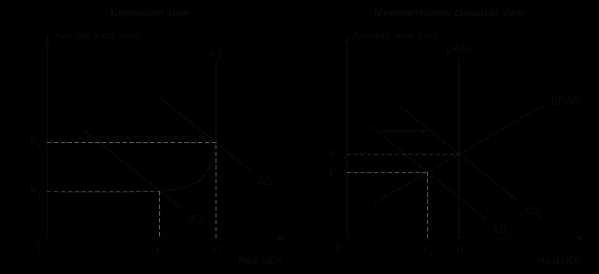
In the Keynesian model, the Keynesian AS curve is horizontal when there is a lot of spare capacity, rises as the economy approaches full capacity, and becomes vertical at Yf. The left-hand panel shows an economy with AD₁ meeting the AS curve at Y₁, in the range where AS is almost flat. Wages and prices are sticky downwards, so the economy can stay at Y₁ for a long time: there is no reliable automatic mechanism that returns it to full employment.
An increase in government spending, or a tax cut that raises consumption and investment, shifts AD₁ to AD₂. Because firms have idle capacity and unemployed workers are available at the going wage, they can raise output without raising costs much. Real GDP rises from Y₁ to Yf, and the average price level rises from P₁ to P₂ only as the economy enters the rising section of the curve where bottlenecks start to appear.
Keynesians therefore see expansionary fiscal policy as an effective cure for a deep recession, and often as the most important one. In their view, a fall in private spending can leave the economy in a long-lasting deflationary gap, and only the government is able to fill the gap in spending. The further the economy is from Yf, the larger the effect on output and the smaller the effect on prices.
In the monetarist/new classical model there is a vertical long-run aggregate supply (LRAS) curve at Yf and an upward-sloping short-run aggregate supply (SRAS) curve. In the right-hand panel, AD₁ meets SRAS at Y₁, below Yf. Expansionary fiscal policy shifts AD to AD₂, and the new short-run equilibrium lies on LRAS at Yf, with a higher price level P₂.
Monetarists/new classical economists accept that this closes the gap, but they question whether it is needed. In their model wages and prices are flexible. With unemployment above the natural rate, money wages fall, SRAS shifts to the right, and the economy returns to Yf by itself at a lower price level. This automatic adjustment makes fiscal intervention unnecessary in the long run, and the policy carries risks: time lags may mean it takes effect after the economy has already recovered, and the deficit adds to debt.
The case against fiscal expansion is strongest when the economy is already at Yf. The figure shows what happens then.
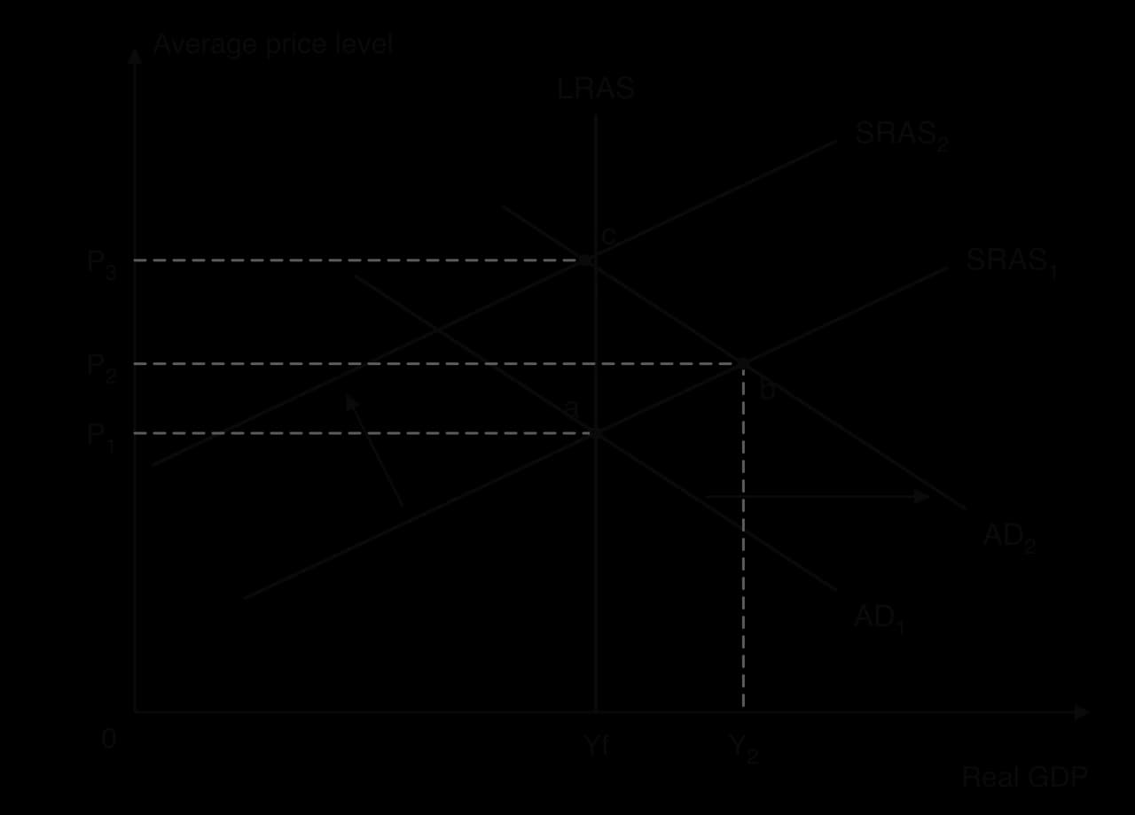
At point b real GDP is above potential output, so unemployment is below its natural rate. Workers are scarce, and as wage contracts are renewed they demand higher money wages to keep up with the rising price level. Higher wages raise firms’ costs, SRAS shifts left from SRAS₁ to SRAS₂, and the economy moves to point c: back at Yf, with the natural rate of unemployment, but with a permanently higher price level. In this view, demand-side policy cannot raise output above Yf for long; only supply-side policies that shift LRAS can do that.
An inflationary gap exists when real GDP is above potential output: firms are working beyond their normal capacity, labour is scarce and prices are rising. Contractionary fiscal policy reduces AD to bring output back to Yf and to ease the pressure on prices.
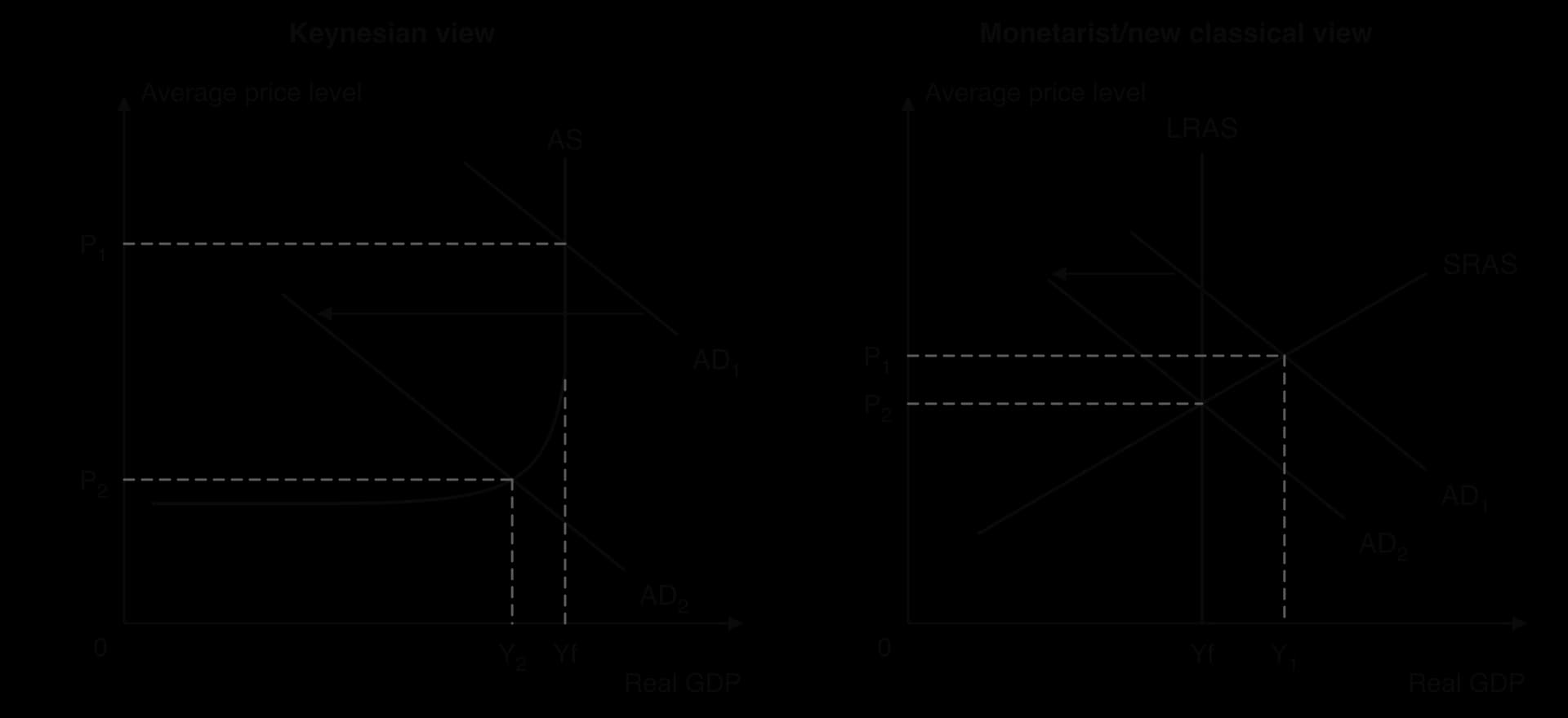
In the Keynesian panel, AD₁ meets the AS curve on its vertical section at Yf: the economy is at full capacity, so any extra spending only raises prices. A cut in government spending or a rise in taxes shifts AD₁ to AD₂. The average price level falls sharply from P₁ to P₂, but because AD₂ meets AS just inside the rising section, real GDP also falls slightly, to Y₂, and some unemployment appears. Keynesians stress that in practice money wages and many prices are slow to fall, so cutting AD tends to reduce the rate of inflation and output, rather than the price level itself.
In the right-hand panel, the monetarist/new classical economy is at Y₁, above Yf, with an inflationary gap. Contractionary fiscal policy shifts AD₁ to AD₂, real GDP falls to Yf and the price level falls from P₁ to P₂. Without the policy, the gap would close by itself in the long run as rising wages shifted SRAS to the left, but at a higher price level. The policy therefore prevents a further rise in prices.
Contractionary fiscal policy is rarely used just to cool a boom, because higher taxes and spending cuts are unpopular and central banks usually take the lead against inflation with higher interest rates. It is used far more often to reduce a large budget deficit. When the economy is weak at the time, the fall in AD can deepen a recession, which is the main criticism of austerity.
Greece after 2009 is the clearest recent case. With a deficit of 15.4% of GDP in 2009 and no access to borrowing from the markets, it cut spending and raised taxes under its rescue programmes, reducing the deficit to 4.1% of GDP by 2013. Real GDP fell every year from 2009 to 2013, unemployment rose from 9.6% to 27.5%, and debt rose from 129% to 181% of GDP, because GDP shrank faster than the debt could be reduced.
Sources: IMF, World Economic Outlook database (2026): general government net lending/borrowing, real GDP growth, unemployment rate and gross debt for Greece.
Keynesian view | Monetarist/new classical view | |
|---|---|---|
Shape of AS | Horizontal, then upward-sloping, then vertical at Yf. | SRAS upward-sloping; LRAS vertical at Yf. |
Wages and prices | Sticky, especially downwards. | Flexible in the long run. |
Can a deflationary gap persist? | Yes, possibly for a long time. | No: falling wages shift SRAS right and output returns to Yf. |
Effect of expansionary fiscal policy | Large rise in real GDP with little inflation when there is spare capacity. | Raises output in the short run only; in the long run mainly raises the price level. |
Role for fiscal policy | Active: the government should fill gaps in private spending. | Limited: keep the budget sound and rely on supply-side policies for growth. |
A rise in government spending raises real GDP by more than the amount spent. The extra spending becomes income for the people who supply the goods and services, and they spend part of that income in turn, creating income for others. This chain of spending is the Keynesian multiplier.
When the government spends an extra $100 million building a new hospital, the construction firms’ workers and owners receive $100 million of extra income: real GDP has risen by $100 million in the first round. If they spend 80% of each extra dollar of income on domestic goods and services, they spend $80 million, which is extra income for shopkeepers, restaurant owners and their staff. These people in turn spend 80% of their extra $80 million, or $64 million, and so on.
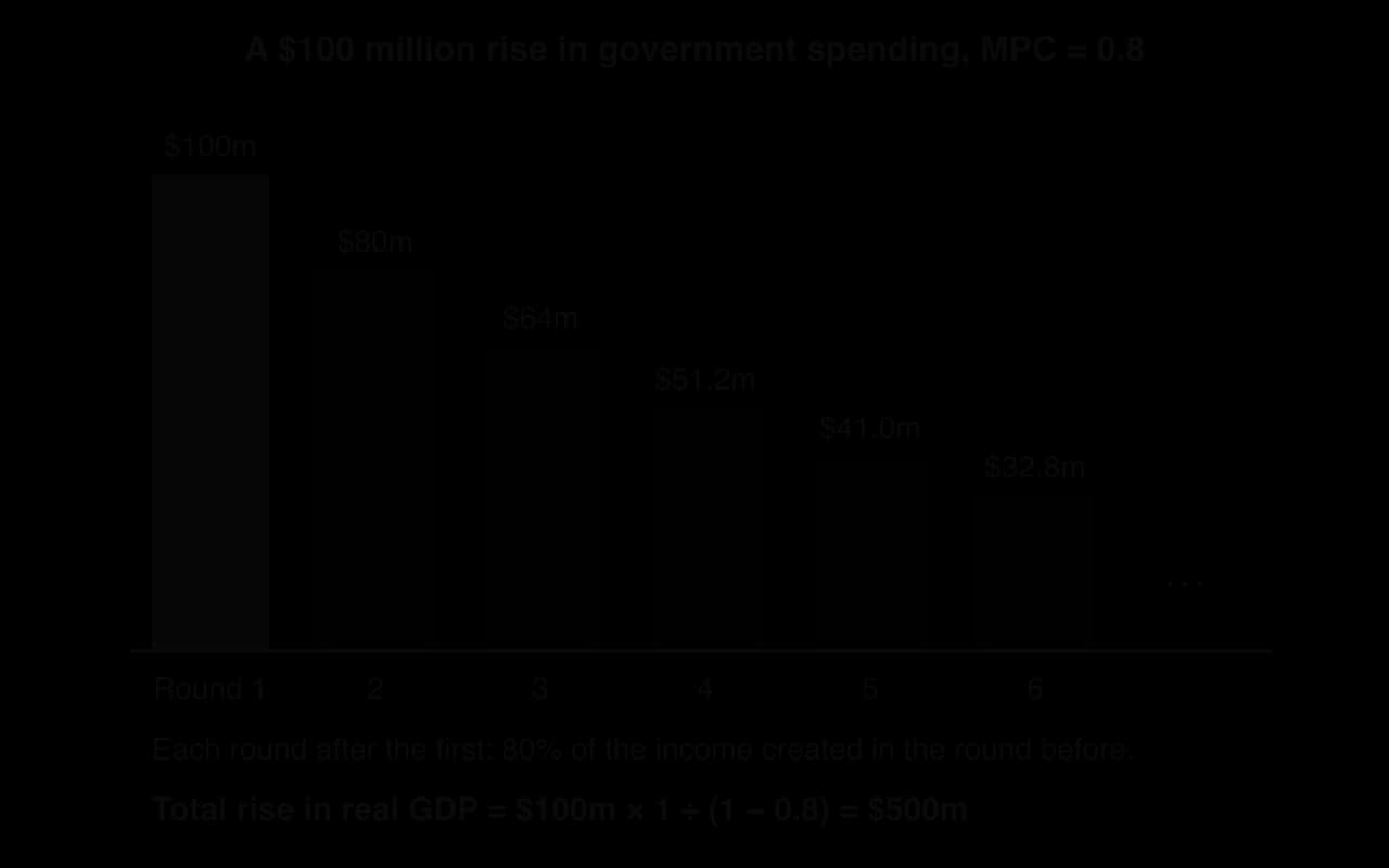
Each round is smaller than the last, because at every step part of the extra income leaks out of the circular flow instead of being spent on domestic output. The rounds add up to a finite total: $100m + $80m + $64m + $51.2m + … = $500 million. The initial injection of $100 million has raised real GDP by $500 million, so the multiplier is 5.
The leakages are the same ones that appear in the circular flow of income: saving, taxes and spending on imports. The more of each extra dollar that leaks out, the smaller each round of spending and the smaller the multiplier.
Four marginal propensities measure how each extra unit of income is used. “Marginal” means they refer to the change in income, not to the total.
The first, the marginal propensity to consume (MPC), measures how much of each extra unit of income is passed on as spending in the next round.
In the simple formula, consumption means spending on domestic output, because only that creates income at home. The other three propensities measure the three leakages: the marginal propensity to save (MPS), the marginal propensity to tax (MPT) and the marginal propensity to import (MPM).
Marginal propensity to tax (MPT): the proportion of an increase in income that is paid in taxes; MPT = ΔT ÷ ΔY. It is high where income taxes are progressive.
Marginal propensity to import (MPM): the proportion of an increase in income that is spent on imports; MPM = ΔM ÷ ΔY. It is high in small, open economies that buy many of their goods abroad.
Every extra dollar of income must be consumed on domestic output, saved, taxed or spent on imports, so the four propensities sum to one.
The size of the multiplier depends only on the share of each extra dollar that is passed on in the next round (the MPC) or, which is the same thing, on the share that leaks out (MPS + MPT + MPM). It can be calculated in either of two equivalent ways.
Once the multiplier is known, the change in real GDP caused by a change in any injection follows directly:
The total change in income is the sum of every round: ΔY = ΔJ + MPC·ΔJ + MPC²·ΔJ + MPC³·ΔJ + … This is a geometric series with first term ΔJ and common ratio MPC. Because MPC is between 0 and 1, the series converges to ΔJ ÷ (1 − MPC).
Since 1 − MPC equals the sum of the leakages (MPS + MPT + MPM), the two forms of the formula always give the same answer.
Leakages differ greatly between economies. A large economy with low taxes, such as the US, buys a smaller share of its goods from abroad than a small open economy such as Ireland or Singapore, where much of any extra spending goes on imports and the multiplier is correspondingly small.
The multiplier can also be shown on an AD/AS diagram. The initial injection shifts AD by the amount of the extra spending; the induced rounds of consumption shift it further.
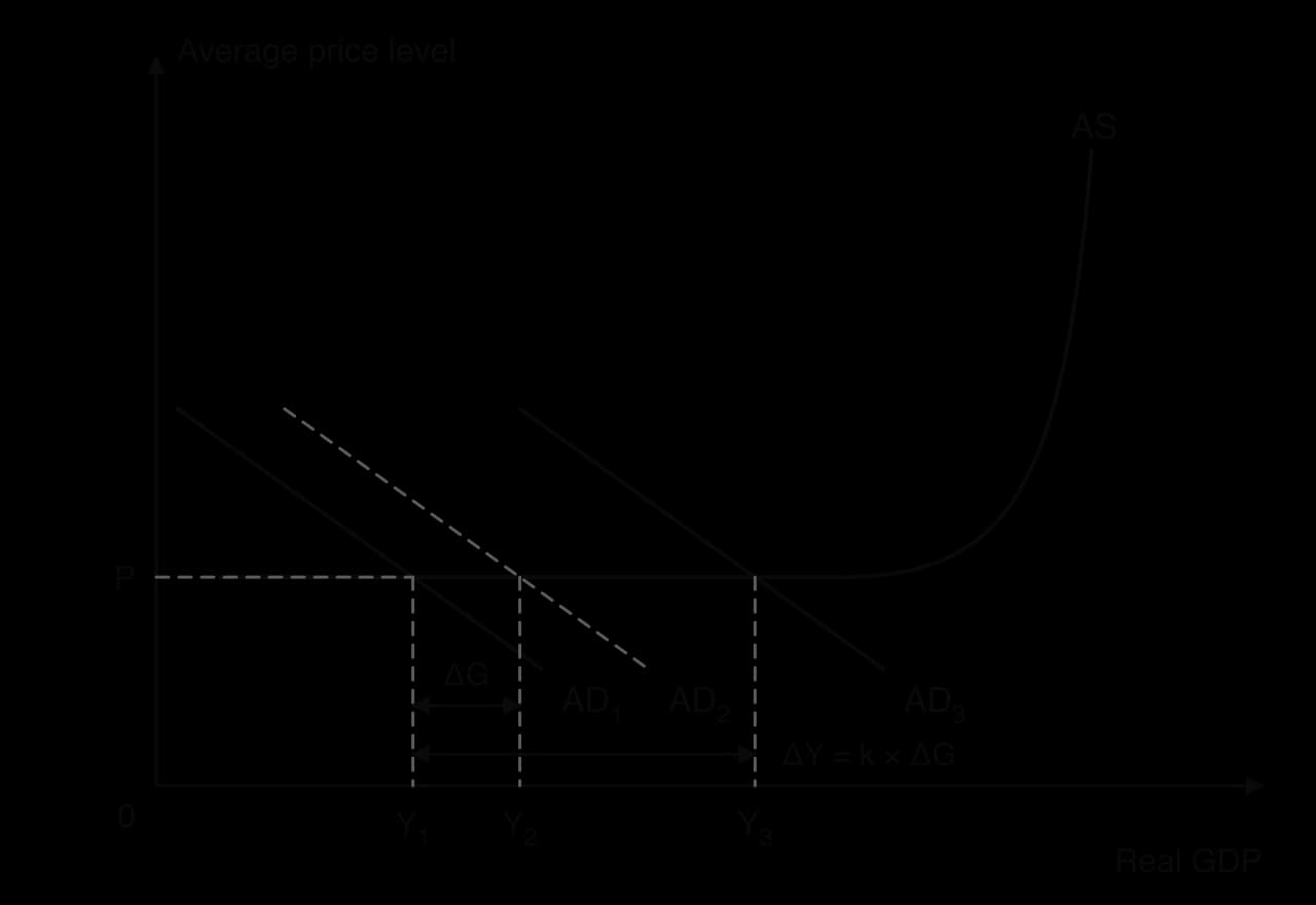
On the horizontal part of the Keynesian AS curve, the whole multiplied rise in AD becomes extra real output. On the rising part, some of it is absorbed by a higher price level instead, so the rise in real GDP is smaller than the simple formula predicts. At Yf the multiplier has no effect on real output at all.
The MPC can be calculated from data on how income and consumption change. If national income rises from $1,000 billion to $1,200 billion and consumption of domestic output rises from $800 billion to $950 billion, then MPC = ΔC ÷ ΔY = 150 ÷ 200 = 0.75, and the multiplier is 1 ÷ 0.25 = 4. The average propensity to consume in the first year (800 ÷ 1,000 = 0.8) is a different number and must not be used.
The simple formula gives an upper limit. In real economies, the multiplier is reduced by rises in the price level, by any rise in interest rates that crowds out private spending, and by households saving more if they expect higher taxes in future to repay the debt. In normal times, estimated multipliers are much smaller than the simple formula suggests.
The size also depends on the state of the economy. When there is a lot of spare capacity, interest rates are near zero and households cannot borrow, multipliers are larger. A 2013 study of the euro area crisis found that growth forecasts had been too optimistic in countries that made larger budget cuts, and concluded that multipliers had been substantially higher than forecasters assumed. Austerity in a deep recession therefore cost more output than expected.
Sources: Olivier Blanchard and Daniel Leigh, “Growth Forecast Errors and Fiscal Multipliers”, IMF Working Paper, January 2013.
 YouTube
Part of fiscal policy works without anyone deciding anything. As the economy moves through the business cycle, tax revenue and some kinds of spending change by themselves, in a direction that dampens the cycle. These are automatic stabilisers.
When real GDP falls, incomes and profits fall, so revenue from income tax, corporate tax and VAT falls. With a progressive income tax, revenue falls faster than incomes, because people move into lower tax brackets and pay a smaller share of their income in tax. Households’ disposable income therefore falls by less than their pre-tax income, which supports consumption.
At the same time, more people lose their jobs and claim unemployment benefits, so transfer payments rise. The benefits replace part of the lost wages and allow the unemployed to keep spending. The budget deficit widens without any new law, and the fall in AD is smaller than it would otherwise have been.
The US in spring 2020 shows the scale this can reach. New claims for unemployment insurance jumped from about 208,000 in the week to 7 March to more than 6.1 million in the week to 4 April, and the number of people receiving benefits peaked at about 23 million in early May. On top of this automatic rise, Congress passed the CARES Act in March 2020, a $2.2 trillion discretionary package that added $600 a week to every unemployment benefit until the end of July and sent $1,200 to most adults.
Sources: US Department of Labor via FRED, series ICSA and CCSA (2020); CARES Act, US Congress (2020).
In a boom the same mechanisms work in reverse. Rising incomes push people into higher tax brackets, so tax revenue rises faster than income and takes spending power out of the economy. Fewer people claim unemployment benefits, so transfer payments fall. The budget moves towards surplus and the rise in AD is held back, reducing the risk of demand-pull inflation.
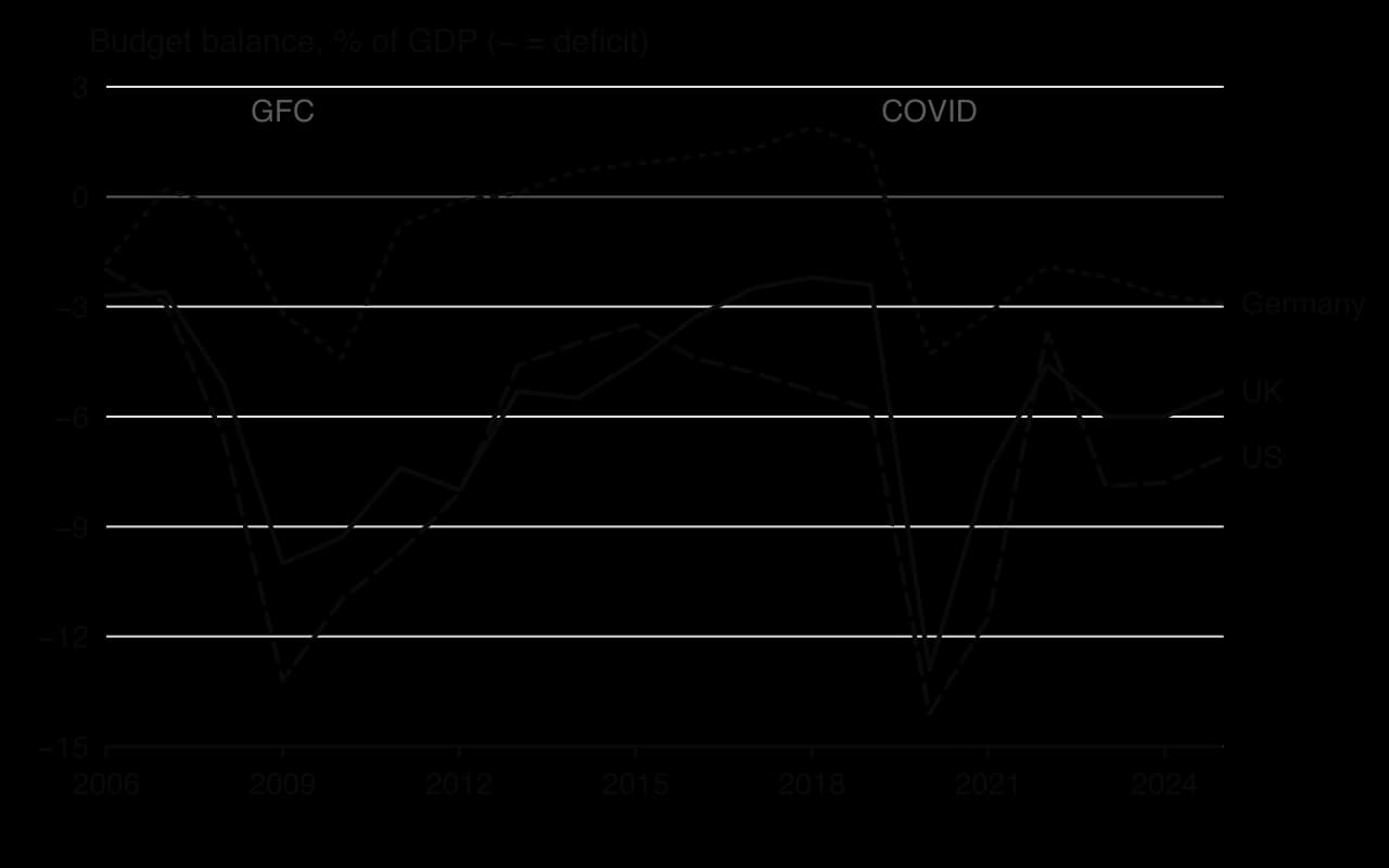
The chart shows how quickly budget balances move with the cycle. In the US, the deficit rose from 2.9% of GDP in 2007 to 13.2% in 2009, and from 5.8% in 2019 to 14.1% in 2020. Germany, which had run surpluses from 2014 to 2019, moved to a deficit of 4.3% in 2020. Part of each swing was discretionary policy and part was automatic, and economists separate the two by estimating a structural (cyclically adjusted) budget balance.
Strengths | Limitations |
|---|---|
No recognition, decision or implementation lag: they react as soon as incomes change. | They reduce fluctuations but cannot remove them or close a large output gap on their own. |
No political decision is needed, so they cannot be delayed by debate or timed for elections. | They widen the deficit in every recession, which adds to debt if surpluses are not run in booms. |
They reverse by themselves in a recovery, so they do not leave a permanent deficit. | Their strength depends on the system: they are weak where taxes are flat and benefits low or absent, as in many low-income economies with large informal sectors. |
They are targeted at those whose incomes have fallen, who are likely to spend the support. | Generous benefits may reduce the incentive to search for work, a supply-side cost. |
Because automatic stabilisers are stronger where taxes are more progressive and benefits more generous, they tend to be strongest in the Nordic countries and Western Europe and weakest in countries where most workers are in the informal economy and pay no income tax and receive no benefits. In those economies, governments must rely much more on discretionary decisions.
Whether fiscal policy works well depends on the type of problem the economy faces, on how the policy is designed and timed, and on the state of the public finances when it is used. Its strengths and its constraints need to be weighed against each other and against monetary policy.
Monetary policy changes interest rates for the whole economy. Fiscal policy can be aimed at particular regions, industries or households: building infrastructure in a poor region, cutting taxes for low-income workers, or supporting a sector hit by a shock. This makes it a tool for equity as well as for demand management.
The UK’s Coronavirus Job Retention Scheme (furlough), announced on 20 March 2020, is an example. The government paid 80% of the wages of employees whose firms could not use them, up to £2,500 a month, so that firms kept workers on their payroll instead of laying them off. About 8.4 million employees were furloughed by late May 2020, and the scheme, which ran until September 2021, cost about £70 billion. Although real GDP fell by 10% in 2020, the unemployment rate rose only from 3.8% in 2019 to 4.6%.
Sources: HM Treasury (2020); House of Commons Library (2021); BBC News (27 May 2020); IMF, World Economic Outlook database (2026).
In a deep recession, monetary policy can lose its power. When interest rates are already close to zero (the zero lower bound), they cannot be cut much further, and when consumer and business confidence is very low, households and firms may not borrow even at very low rates. Government spending does not depend on anyone’s willingness to borrow: it adds to AD directly. This is why governments turned to large fiscal packages in both 2008–09 and 2020.
Spending on infrastructure, education and health raises AD in the short run and can also improve the quantity and quality of the factors of production, shifting LRAS to the right in the long run. Fiscal policy of this kind has supply-side effects, which can allow growth without inflation.
Fiscal decisions are taken by politicians who must win elections. Tax cuts and new spending are popular; tax rises and spending cuts are not. Governments therefore tend to run expansionary policy readily in downturns but find it hard to tighten in booms, which can leave a deficit even in good years and a rising debt over time. Spending may also be timed for elections or directed to politically important areas rather than to where the economic need is greatest.
Time lags are the delays between a problem appearing in the economy and the policy taking full effect. Fiscal policy is subject to several of them, one after another.
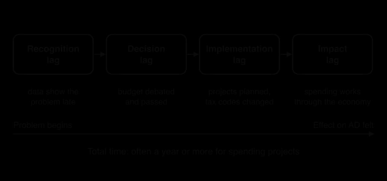
Recognition lag: GDP data are published weeks after each quarter ends and are often revised, so a recession may be recognised only months after it began.
Decision lag: a budget must be drafted, debated and voted on; in some systems, such as the US, the executive and the legislature may disagree for months.
Implementation lag: changing tax codes takes time, and capital projects need planning, land and contracts before spending starts.
Impact lag: the multiplier rounds and the response of firms and households take time to work through the economy.
If the lags are long, a stimulus intended to fight a recession may take effect during the recovery and add to inflation, making fluctuations larger rather than smaller. Tax changes and transfer payments usually act faster than capital spending, which is why many stimulus packages favour them.
Expansionary fiscal policy usually means a larger deficit and more debt. Debt can be sustained as long as the government can pay the interest on it and lenders trust it to do so. When debt is high, debt servicing costs take a growing share of revenue, leaving less for public services; lenders may demand higher interest rates, and a fall in a country’s credit rating can make borrowing more expensive still. A government that is already highly indebted has less room to stimulate the economy in the next recession.
To make borrowing more credible, many governments adopt a fiscal rule. Germany’s “debt brake”, written into its constitution in 2009, limited the federal government’s structural deficit to 0.35% of GDP from 2016. In March 2025 the Bundestag and Bundesrat amended it to exempt defence spending above 1% of GDP and to create a special infrastructure fund of €500 billion, allowing much higher borrowing for defence and public investment.
Sources: Basic Law of the Federal Republic of Germany, Articles 109, 115 and 143h; Bundestag and Bundesrat votes of 18 and 21 March 2025.
Leakages to imports. In open economies much of any stimulus is spent on imports, so it raises AD in other countries more than at home and can widen the current account deficit.
Confidence and expectations. If households expect a tax cut to be temporary, or expect higher taxes later to repay the debt, they may save it rather than spend it.
Inflation risk. Near full capacity, a stimulus raises the price level more than output.
Opportunity cost. Money spent on one programme, such as a fuel subsidy, cannot be spent on another, such as schools.
Opportunity cost became pressing during the 2026 oil price shock. Malaysia sells RON95 petrol to eligible citizens at a subsidised RM1.99 a litre; when conflict in West Asia drove up world oil prices, the monthly cost of fuel subsidies rose from about RM700 million to about RM5 billion by May 2026. From April 2026 the government cut each person’s subsidised monthly quota from 300 to 200 litres, choosing to limit the cost to the budget while still protecting most users.
Sources: Free Malaysia Today (26 March 2026); The Vibes (4 May 2026), reporting the Prime Minister.
A larger deficit must be financed by borrowing. When the government borrows by selling bonds, it competes with firms and households for the funds that savers make available. If the extra demand for funds pushes up interest rates, private investment and consumption financed by borrowing fall, offsetting part of the rise in AD. This is crowding out.
Crowding out is shown in the market for loanable funds, where the supply of loanable funds comes from saving and the demand comes from firms, households and the government that want to borrow. The price in this market is the real interest rate.
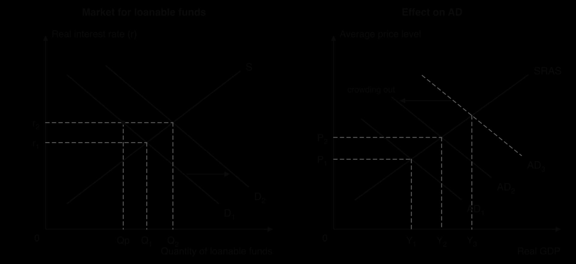
In the left-hand panel, the government’s extra borrowing shifts the demand for loanable funds from D₁ to D₂. The real interest rate rises from r₁ to r₂. At the higher rate, the total quantity of funds lent rises to Q₂, because saving rises, but private borrowers now take only Qp instead of Q₁: the gap Q₁ − Qp is private investment and borrowing that no longer happens.
The right-hand panel shows the effect on the economy. Without crowding out, the rise in government spending would shift AD from AD₁ to AD₃. Because higher interest rates reduce private investment and spending on durable goods, AD shifts only to AD₂, and real GDP rises only to Y₂. In the extreme case that private spending falls by as much as government spending rises, crowding out is complete and fiscal policy has no effect on AD.
Monetarist/new classical economists argue that crowding out is large, especially when the economy is close to full employment and when the government borrows heavily year after year. Keynesians argue that it is small in a recession. With many unemployed resources and weak investment, firms are not competing strongly for funds, households are saving more, and the central bank is usually keeping interest rates low, so government borrowing does not push rates up much.
Evidence fits the Keynesian view for deep recessions: in 2009 and 2020, government borrowing in the US, the UK and the euro area rose enormously while long-term interest rates stayed low or fell, partly because central banks were buying government bonds through quantitative easing. In normal times, and in countries whose lenders doubt the government’s ability to repay, the risk of crowding out is much greater.
Objective | Strengths of fiscal policy | Limitations |
|---|---|---|
Economic growth | Raises AD quickly in a recession; capital spending on infrastructure and education raises potential output. | Short-run boost only if spending is wasteful; high debt and crowding out may reduce private investment and future growth. |
Low unemployment | Directly creates jobs through public projects; can be aimed at regions and sectors with high unemployment; (HL) automatic stabilisers support demand. | Reduces cyclical unemployment only; structural unemployment needs supply-side measures; time lags may delay the effect. |
Low and stable inflation | Contractionary policy can reduce demand-pull inflation; (HL) automatic stabilisers restrain booms. | Politically hard to raise taxes or cut spending; ineffective against cost-push inflation, where cutting AD deepens the fall in output. |
Fiscal policy is strongest against a deep recession caused by a collapse in private demand, especially when interest rates are already at the zero lower bound, when the government has room to borrow, and when it can spend quickly on useful projects. It is weakest against inflation, where its political difficulty and long lags make monetary policy the usual first choice, and when debt is already so high that more borrowing raises interest rates or undermines confidence.
Fiscal policy | Monetary policy | |
|---|---|---|
Who decides | Government and legislature | Central bank, usually independent |
Speed of decision | Slow: budgets need debate and votes | Fast: rate-setting meetings several times a year |
Targeting | Can target sectors, regions and income groups | Affects the whole economy through interest rates |
In a deep recession | Effective: spending adds to AD directly | Limited near the zero lower bound and when confidence is low |
Main cost | Deficits and debt; political pressure | Distributional effects on borrowers and savers; asset prices |
Most economists now see the two policies as complements. In normal times, central banks manage demand and fiscal policy is left to automatic stabilisers and to the longer-term goals of public services, equity and investment. In deep recessions both are used together, with fiscal policy doing more of the work.
When the global financial crisis hit in late 2008, China’s exports collapsed as demand in the US and Europe fell, and growth slowed sharply. On 9 November 2008 the State Council announced a package of 4 trillion yuan (about US$586 billion) of spending on infrastructure and social welfare to be completed by the end of 2010. China’s nominal GDP in 2008 was about 32.4 trillion yuan, so the package was equal to about 12% of one year’s GDP, spread over two years.
Use of funds in the revised plan of March 2009 | Trillion yuan |
|---|---|
Public infrastructure: railways, roads, irrigation, airports | 1.50 |
Reconstruction after the 2008 Sichuan earthquake | 1.00 |
Rural development | 0.37 |
Technology and industrial upgrading | 0.37 |
Energy saving, emissions reduction and environmental projects | 0.21 |
Education, culture and family planning | 0.15 |
Other items, including low-cost housing (remainder) | 0.40 |
Sources: National Development and Reform Commission plan of 6 March 2009, as reported in “Chinese economic stimulus program”, Wikipedia (accessed October 2026); remainder calculated.
The theory of expansionary fiscal policy predicts what followed. The package was almost all capital expenditure, which adds directly to G and I, and China had a great deal of spare capacity in construction and heavy industry once export orders had dried up, so in Keynesian terms AD shifted right along a fairly flat section of the AS curve. Investment (gross capital formation) rose from 42.0% of GDP in 2008 to 44.9% in 2009 and 46.1% in 2010. Real GDP grew by 9.4% in 2009 while world output shrank and advanced economies contracted by 3.4%.
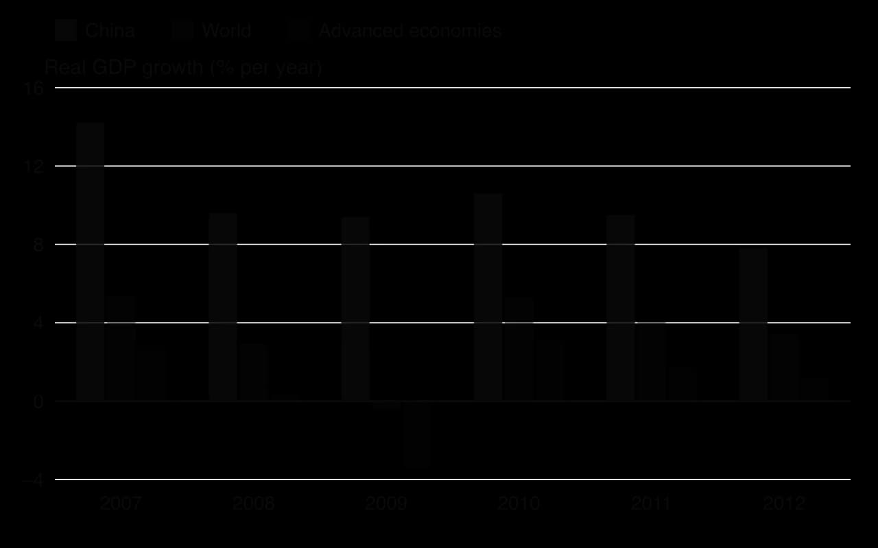
Several features made the stimulus fast and powerful. Spending was channelled through local governments and state-owned enterprises, so decisions could be taken quickly and the decision lag was short. State-owned banks were instructed to lend: bank loans to local governments rose by about 70% between the end of 2008 and the end of 2009. Because the state directed credit to the projects, and the central bank kept interest rates low, there was little crowding out of the kind the loanable funds model predicts.
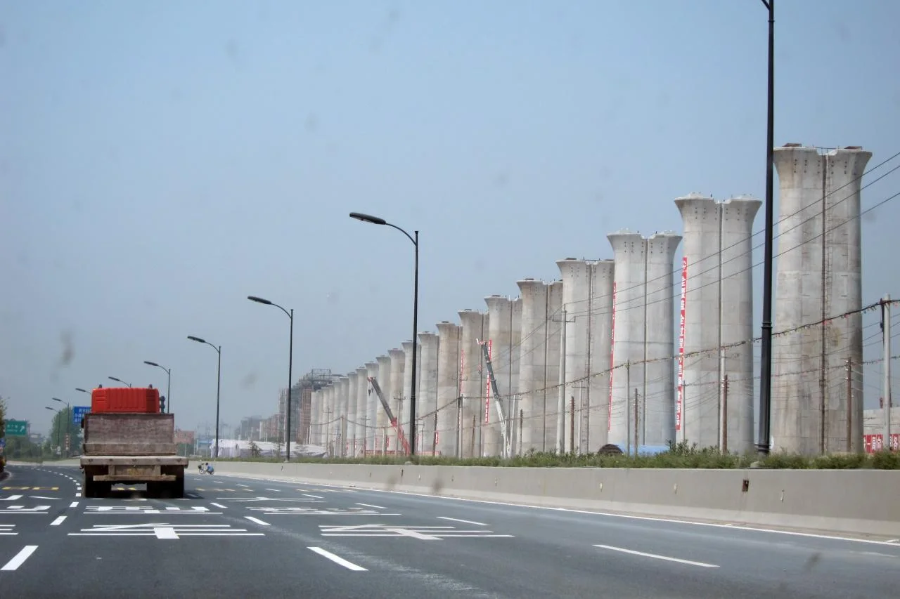
The costs appeared later and show the constraints on fiscal policy. The central government provided only about 1.2 trillion yuan of the 4 trillion; local governments were expected to find most of the rest. They were not allowed to borrow directly, so they set up local government financing vehicles (LGFVs) that borrowed from banks on their behalf.
As a result the official general government deficit rose only to 1.7% of GDP in 2009, while borrowing outside the budget grew rapidly. Local government debt reached about 7.7 trillion yuan in 2010 and 17.9 trillion yuan by 2013; by the end of 2023 LGFV debt was estimated at about US$8 trillion, or 47% of GDP.
The rapid spending also had efficiency costs. Some projects earned too little to repay their loans, the investment boom is widely blamed for excess capacity in heavy industry, and credit flowed into property. Inflation, which was −0.7% in 2009, rose to 5.4% in 2011, and the authorities tightened lending from 2010 to cool the property market.
The case shows both sides of expansionary fiscal policy. It was effective as demand management: AD was supported quickly and on a large scale, and the multiplier worked through a large domestic economy with spare capacity. Its limits were sustainability and efficiency: the debt was hidden off the budget, much of the investment had low returns, and the debts of local governments became a constraint on China’s economy more than a decade later. A smaller, more transparent package, financed on the central government’s budget, might have achieved most of the gains with fewer of the costs.
Sources: IMF, World Economic Outlook database (2026): real GDP growth, inflation, general government net lending/borrowing; World Bank, World Development Indicators (2026): GDP (current LCU), gross capital formation (% of GDP); State Council announcement (2008); “Local government financing vehicle”, Wikipedia (accessed October 2026), citing China’s National Audit Office (2013) and the IMF (2024).
Fiscal policy appears in all papers. Paper 1 questions usually ask you to explain how fiscal policy can close a gap, with a diagram, and then to evaluate it with real-world examples. Paper 2 can ask you to define terms such as budget deficit or expansionary fiscal policy, to explain a policy in the text with an AD/AS diagram, and to discuss its effectiveness using the data. At HL, Paper 3 regularly includes multiplier calculations and a policy recommendation in which fiscal policy is one option.
Paper 2-style items (hypothetical text about a country whose government cuts income tax and raises spending on rail during a recession):
Define the term expansionary fiscal policy indicated in bold in the text. [2]
Using the data, calculate the government’s budget balance in 2025 as a percentage of GDP (revenue $310 billion, spending $355 billion, GDP $1,500 billion). [2]
Using an AD/AS diagram, explain how the income tax cut could reduce cyclical unemployment. [4]
Using information from the text/data and your knowledge of economics, evaluate the government’s decision to use fiscal policy to end the recession. [15]
1. An increase in government spending and/or a reduction in taxes (1 mark) intended to increase aggregate demand / economic activity (1 mark).
2. Balance = 310 − 355 = −$45 billion; −45 ÷ 1,500 × 100 = a deficit of 3% of GDP. Show the working and the sign.
3. Diagram: correctly labelled axes, AD₁ to AD₂, Y₁ to Y₂ and P₁ to P₂ (2 marks). Explanation: lower income tax raises disposable income and consumption, so AD rises; firms raise output and hire more workers, so cyclical unemployment falls (2 marks).
4. Sketch: define; explain with a diagram; then use the text’s figures (size of the stimulus relative to GDP, the debt level, the interest rate, how quickly the rail spending can start) to weigh strengths (direct effect on AD, targeting, multiplier) against constraints (time lags for rail, debt sustainability, inflation if the economy is near Yf, leakages to imports). End with a judgment tied to the country’s situation.
Fiscal policy is the use of government spending and taxation to influence aggregate demand; it is set by the government, not the central bank.
Revenue comes from direct and indirect taxes, sales by state-owned enterprises and sales of assets; spending is current, capital or transfer payments.
Expansionary fiscal policy (higher G, lower taxes) shifts AD right to close a deflationary gap; contractionary policy shifts AD left to close an inflationary gap or cut a deficit.
Keynesians see fiscal policy as essential in a deep recession; monetarists/new classical economists expect output to return to Yf by itself and warn that stimulus raises prices in the long run.
HL: the multiplier k = 1 ÷ (1 − MPC) = 1 ÷ (MPS + MPT + MPM) makes the change in real GDP a multiple of the change in an injection.
HL: automatic stabilisers (progressive taxes, unemployment benefits) dampen the cycle without new decisions; crowding out can reduce the effect of government borrowing.
Strengths: targeting and effectiveness in deep recessions. Constraints: political pressure, time lags and sustainable debt.
I can describe the four sources of government revenue and the three types of government spending.
I can distinguish a budget deficit from government debt.
I can explain the six goals of fiscal policy and how fiscal tools affect C, I and G.
I can draw and explain expansionary and contractionary fiscal policy on Keynesian and monetarist/new classical AD/AS diagrams.
I can explain the multiplier and calculate it from the MPC or from the leakages (HL).
I can calculate the change in real GDP from a change in investment, government spending or exports (HL).
I can draw and explain the crowding out diagram (HL).
I can explain how progressive taxes and unemployment benefits act as automatic stabilisers (HL).
I can evaluate fiscal policy using strengths, constraints and a real-world example, and reach a judgment.
0 |
0 |
The work does not reach a standard described by the descriptors below. |
1 | 1–2 | Little understanding of the specific demands of the question. Relevant economic theory is stated but not relevant. Economic terms are stated but not relevant. |
2 | 3–4 | Some understanding of the specific demands of the question. Relevant economic theory is described. Some relevant economic terms are included. |
3 | 5–6 | The specific demands of the question are understood but only partially addressed. Relevant economic theory is partly explained. Some relevant terms are used appropriately. Where appropriate, relevant diagram(s) are included. |
4 | 7–8 | The specific demands of the question are understood and addressed. Relevant economic theory is explained. Relevant terms are used mostly appropriately. Where appropriate, relevant diagram(s) are included and explained. |
5 | 9–10 | The specific demands of the question are understood and addressed. Relevant economic theory is fully explained. Relevant terms are used appropriately throughout. Where appropriate, relevant diagram(s) are included and fully explained. |
Using real-world examples, discuss the effectiveness of expansionary fiscal policy in reducing unemployment.
15 marks
Answers may include:
Terminology: expansionary fiscal policy, government spending, taxation, aggregate demand (AD), deflationary (recessionary) gap, cyclical (demand-deficient) unemployment, budget deficit, government (national) debt.
Explanation: higher government spending and lower taxes increase injections and reduce leakages, raising AD; firms increase output and hire more workers, reducing cyclical unemployment; a multiplier effect may magnify the impact (HL candidates may refer to the Keynesian multiplier).
Diagram(s): AD/AS diagram showing AD shifting right, closing a deflationary (recessionary) gap and raising real GDP; circular flow diagram with a larger injection.
Synthesis/evaluation: effective against cyclical unemployment but not structural, frictional or seasonal unemployment; time lags in planning and implementation; effectiveness depends on the size of the spare capacity (close to full employment, AD increases mainly raise the price level); rising budget deficits and debt may limit the scope for policy and raise interest rates; a high marginal propensity to import weakens the effect; political constraints; contrast with monetary policy when interest rates are already low; a reasoned conclusion.
Examples: the US American Recovery and Reinvestment Act (2009) during the global financial crisis; China's large stimulus package of 2008–2009 focused on infrastructure; job-retention and furlough schemes in 2020 (such as the UK Coronavirus Job Retention Scheme); Japan's repeated fiscal stimulus in the 1990s and its rising public debt.
N.B. Terminology, theory, diagrams and examples given in part (a) and referred to in part (b) should be rewarded.
Examiners should be aware that candidates may take a different approach which, if appropriate, should be rewarded.
Markbands (best fit)
Level | Marks | Descriptor |
|---|---|---|
0 | 0 | The work does not reach a standard described by the descriptors below. |
1 | 1–3 | Little understanding of the specific demands of the question. Theory is stated but not relevant. Terms are not relevant. No synthesis or evaluation. Real-world examples are identified but not relevant. |
2 | 4–6 | Some understanding of the demands. Relevant theory is described. Some relevant terms are included. Synthesis or evaluation is superficial. A relevant real-world example is identified. |
3 | 7–9 | The demands are understood but only partially addressed. Theory is partly explained. Some terms are used appropriately. Relevant diagram(s) are included where appropriate. Synthesis or evaluation is appropriate but lacks balance. Example(s) are identified and partly developed in context. |
4 | 10–12 | The demands are understood and addressed. Theory is explained. Terms are used mostly appropriately. Diagram(s) are included and explained. Synthesis or evaluation is appropriate and mostly balanced. Example(s) are identified and developed in the context of the question. |
5 | 13–15 | The demands are understood and addressed. Theory is fully explained. Terms are used appropriately throughout. Diagram(s) are included and fully explained. Synthesis or evaluation is effective and balanced. Example(s) are identified and fully developed to support the argument. |
Read the extract and answer the questions that follow.
Text A — A shrinking flow of income in Tarvesh
[1] Tarvesh is a high-income economy in northern Europe with a large manufacturing sector. Around 45 % of its manufactured goods are sold to its neighbour, Holvenia.
[2] In 2025, a recession in Holvenia reduced spending on Tarvesh's exports. Exports are an injection into Tarvesh's circular flow of income, while saving, taxes and imports are leakages. At the same time, Tarvesh's households became more cautious and increased their saving. Estimates for 2025 are shown in Table 1.
[3] The finance minister has said that the government will 'not stand by while the economy shrinks', but has not yet announced any measures.
Table 1: Leakages and injections in Tarvesh, 2025 (TVS billion)
Item | Value |
|---|---|
Saving | 42 |
Taxes | 65 |
Imports | 58 |
Investment | 38 |
Government spending | 70 |
Exports | 49 |
Define the term injection indicated in bold in the text (Text A, paragraph 2).
2 marks
Using information from Table 1, calculate the difference between total leakages and total injections in Tarvesh in 2025.
2 marks
Using your answer to (b)(i), state whether Tarvesh's national income is likely to rise or fall.
1 mark
Using a circular flow of income diagram, explain how the recession in Holvenia is likely to affect household incomes in Tarvesh (Text A, paragraphs 1 and 2).
4 marks
Explain two measures the government of Tarvesh could use to bring leakages and injections back into balance at a higher level of national income (Text A, paragraph 3).
4 marks
Read the extract and answer the questions that follow.
Text A — Clinics or aircraft? Mirelland's budget dilemma
[1] Mirelland is an upper-middle-income economy in South America. Its government has set aside MRL 480 million (Mirelland lira) for new capital spending in 2026, to be divided between rural health clinics and military aircraft. Scarcity of public funds means that it cannot satisfy both the health ministry and the defence ministry in full.
[2] Each new rural clinic, fully equipped, costs MRL 12 million. Each military aircraft costs MRL 96 million. The defence ministry has requested three aircraft.
[3] Health campaigners point out that infant mortality in rural districts is twice the national average, while the defence ministry argues that national security is a public good that only the government can provide.
Define the term scarcity indicated in bold in the text (Text A, paragraph 1).
2 marks
Using information from Text A, paragraph 2, calculate the opportunity cost, in rural clinics, of buying the three aircraft requested by the defence ministry.
2 marks
Using information from Text A, determine the maximum number of rural clinics that could be built if no aircraft were bought.
1 mark
Using a production possibilities curve (PPC) diagram, explain the choice faced by Mirelland's government (Text A, paragraphs 1 and 2).
4 marks
Explain two reasons why national security may be provided by the government rather than by the market (Text A, paragraph 3).
4 marks