 YouTube
Calculate contribution, break-even quantity, margin of safety, target profit output and target price, construct and read a break-even chart, show the effects of price and cost changes, and evaluate break-even analysis.
Each is in the Business glossary, with every other term in the subject.
A decision-making tool that uses fixed costs, variable costs and selling price to find the output at which total revenue equals total cost, and the profit or loss at other outputs.
A graph showing a business's fixed cost, total cost and total revenue lines against output, on which the break-even point is where the total revenue and total cost lines intersect.
The level of output at which total revenue equals total cost, so that the business makes neither a profit nor a loss; fixed costs divided by contribution per unit.
The value of sales at which total revenue equals total cost; the break-even quantity multiplied by the selling price.
The difference between sales revenue and variable costs, which is used first to pay a business's fixed costs and then provides its profit.
The selling price of one unit minus its variable cost per unit; the amount each unit sold adds towards fixed costs and then profit.
The percentage of a transport operator's available capacity, such as the seats on a flight, that is actually sold or used in a period.
Distinguish between contribution per unit and total contribution, and calculate both.
Calculate the break-even quantity, break-even revenue and the profit or loss at a given level of output.
Construct a fully labelled break-even chart from data, step by step.
Identify the break-even point, the profit and loss areas and the margin of safety on a break-even chart.
Calculate the margin of safety, the target profit output and the target price.
Analyse the effects of changes in price, variable costs and fixed costs on the break-even quantity, profit and margin of safety, using charts and calculations.
Evaluate break-even analysis as a decision-making tool.
Break-even analysis is a method of finding the level of output at which a business covers all of its costs, so that it makes neither a profit nor a loss. From that one figure managers can work out how far sales can fall before the business makes a loss, how many units it must sell to reach a profit target, and what price it would need to charge. Start-ups use it in their business plans, and established firms use it to test pricing and cost decisions before they make them.
Break-even analysis is closely linked to change. A rise in the price of fuel, a new rent agreement or a decision to cut prices all move the break-even point, and the tool shows by how much. It also raises questions of ethics and sustainability: a business under pressure to reach break-even may be tempted to cut variable costs by paying suppliers less or by using cheaper, less sustainable materials.
75 exam-style questions on this subtopic, written in the style of the IB papers. The first has its markscheme open. Counted on
Prairie Oat Co.
Prairie Oat Co. (POC) is a private limited company in Saskatoon, Canada, that makes oat drinks from oats grown by local farmers. It plans to launch a new barista-style oat drink in 1-litre cartons for coffee shops and supermarkets across western Canada. The market for plant-based drinks is growing, but it is dominated by two international brands that sell their cartons for about CAD 3.80.
POC’s marketing team has prepared forecasts for two pricing strategies, shown in Table 1. The fixed costs of the new production line are CAD 700 000 a year, and the variable cost is CAD 1.70 per carton under either strategy.
Table 1: Forecasts for the first year of the new oat drink
Premium pricing | Penetration pricing | |
|---|---|---|
Price per carton (CAD) | 4.50 | 3.20 |
Forecast sales (cartons) | 400 000 | 750 000 |
POC’s factory can produce up to 800 000 cartons a year. Its brand is well known for its local sourcing.
Using Table 1, calculate the contribution per carton under each pricing strategy (show all your working).
2 marks
Premium: CAD 4.50 − CAD 1.70 = CAD 2.80
Penetration: CAD 3.20 − CAD 1.70 = CAD 1.50
The official deck for this part of the syllabus.
What is break-even analysis?
What is the break-even quantity (break-even point)?
With a free account, Augment remembers where you stopped and what you have practiced.
The regions of a break-even chart between the total revenue and total cost lines: the loss area left of the break-even point and the profit area to its right.
The selling price per unit needed to achieve a target profit at a given level of output; fixed costs plus target profit divided by output, plus variable cost per unit.
The level of profit that a business sets out to achieve in a given period.
The level of output a business must sell to achieve a chosen target profit; fixed costs plus target profit, divided by contribution per unit.
The contribution made by all the units sold in a period, equal to contribution per unit multiplied by quantity sold, or total revenue minus total variable costs.
Scope: Break-even analysis is part of operations management at SL and HL. Both levels calculate contribution, the break-even quantity, profit or loss, the margin of safety, the target profit output and the target price; construct and read break-even charts; show the effects of changes in price and cost graphically and by calculation; and evaluate the limitations of the tool. The same content applies at SL and HL.
Every business has two kinds of cost. Fixed costs stay the same whatever the level of output in a given period: rent, insurance, salaries of permanent staff, loan interest. Variable costs change in direct proportion to output: raw materials, packaging, piece-rate wages, the energy used by each machine-hour. Total cost is the sum of the two, and total revenue is the price multiplied by the number of units sold.
When a business sells only a few units, total revenue is smaller than total cost, because the fixed costs have to be paid however little is sold. As output rises, each extra unit sold brings in more than it costs to make, and the gap closes. At one level of output total revenue exactly equals total cost. That level is the break-even point, and every unit sold beyond it adds to profit.
Break-even analysis rests on a few simplifying assumptions. The selling price is the same for every unit sold, the variable cost per unit is constant, fixed costs do not change within the range of output studied, and everything that is produced is sold. These assumptions make the cost and revenue lines straight, which is what makes the calculations simple, but each of them also limits how far the results can be trusted.
Item | Meaning | Example for a bottle maker |
|---|---|---|
Fixed costs (FC) | Costs that do not change with output in the period | Factory rent, machine lease, managers’ salaries |
Variable cost per unit | The cost of producing one more unit | Steel, lid, packaging and labelling for one bottle |
Total variable costs (TVC) | Variable cost per unit × output | $10 × 7,000 bottles = $70,000 |
Total cost (TC) | FC + TVC | $60,000 + $70,000 = $130,000 |
Total revenue (TR) | Price × quantity sold | $25 × 7,000 bottles = $175,000 |
Profit (or loss) | TR − TC | $175,000 − $130,000 = $45,000 |
The table uses the example of AquaLoop, a small manufacturer of reusable steel water bottles (hypothetical data). AquaLoop sells each bottle for $25, the variable cost of making one is $10, its fixed costs are $60,000 a year, it forecasts sales of 7,000 bottles this year, and its factory can make at most 8,000 bottles a year.
Some costs are partly fixed and partly variable. A semi-variable cost such as a phone contract or a delivery van’s running costs has a fixed element and an element that rises with use. For break-even analysis the two parts are separated: the fixed part is added to fixed costs and the variable part to the variable cost per unit.
The key to break-even analysis is the idea of contribution. When AquaLoop sells one bottle for $25, $10 of that money pays for the materials and labour used to make it. The remaining $15 is left over. It is not yet profit, because the business still has $60,000 of fixed costs to pay. Instead, each $15 is a contribution towards those fixed costs, and once they are fully covered, each further $15 is a contribution to profit.
For AquaLoop the contribution per unit is $25 − $10 = $15. The figure measures how much each sale helps the business. A product with a high contribution per unit, such as a luxury watch, needs to sell fewer units to cover a given amount of fixed costs than a product with a low contribution per unit, such as a bottle of water.
Total contribution is the pool of money available to pay the fixed costs. If AquaLoop sells 7,000 bottles, its total contribution is $15 × 7,000 = $105,000. The same answer comes from total revenue minus total variable costs: $175,000 − $70,000 = $105,000. Whatever is left of the total contribution after the fixed costs have been paid is profit.
With sales of 7,000 bottles, AquaLoop’s profit is $105,000 − $60,000 = $45,000. This is the same figure as total revenue minus total cost, reached by a shorter route. The contribution method is quicker whenever price and variable cost per unit are known, and it makes clear why profit rises so fast once fixed costs are covered.
The table shows how AquaLoop’s total contribution builds up against its fixed costs as sales rise. Below 4,000 bottles the total contribution does not cover the fixed costs and the business makes a loss; at 4,000 it covers them exactly; above 4,000 every bottle adds $15 to profit.
Bottles sold | Total contribution ($) | Fixed costs ($) | Profit or loss ($) |
|---|---|---|---|
0 | 0 | 60,000 | (60,000) |
2,000 | 30,000 | 60,000 | (30,000) |
4,000 | 60,000 | 60,000 | 0 |
6,000 | 90,000 | 60,000 | 30,000 |
7,000 | 105,000 | 60,000 | 45,000 |
8,000 | 120,000 | 60,000 | 60,000 |
The two measures answer different questions. Contribution per unit shows how much each sale is worth to the business, so it is used to compare products, to judge a price change and to calculate the break-even quantity. Total contribution shows how much the whole volume of sales is worth, so it is compared with fixed costs to find the profit for the period.
A product can have a high contribution per unit but a low total contribution, if it sells in small numbers, and the reverse is also true. A supermarket earns a small contribution on each loaf of bread but sells so many loaves that bread brings in a large total contribution. A furniture maker may earn several hundred dollars of contribution on one hand-made table but sell only a few tables a month.
Uber shows how important total contribution is in a business with high fixed costs. Its technology platform, research and corporate costs do not rise in proportion to the number of trips, so total contribution had to grow a long way before it covered them. Uber reported an operating loss in every year from 2017 to 2022, then its first annual operating profit, $1.1 billion, in 2023, which rose to $5.6 billion in 2025 as the number of trips kept growing.
Sources: Uber Technologies, Form 10-K annual reports 2017–2025 (SEC filings); Uber, fourth quarter and full year 2023 results, 7 February 2024.
The tutor2u video explains contribution and uses it to find the break-even point, the same method as in the worked example.
YouTubeThe break-even quantity is the number of units a business must sell for total revenue to equal total cost. The contribution idea gives a direct way to calculate it. Each unit sold contributes a fixed amount towards the fixed costs, so the business breaks even when it has sold enough units for their total contribution to equal the fixed costs.
For AquaLoop the break-even quantity is $60,000 ÷ $15 = 4,000 bottles. The answer can be checked by working out total revenue and total cost at that output: total revenue is $25 × 4,000 = $100,000, and total cost is $60,000 + ($10 × 4,000) = $100,000. Revenue equals cost, so profit is zero.
The formula shows the two ways a business can lower its break-even quantity. It can reduce its fixed costs, the top of the fraction, for example by moving to cheaper premises. Or it can raise its contribution per unit, the bottom of the fraction, either by raising the price or by cutting the variable cost per unit. A business with high fixed costs and a low contribution per unit has a high break-even quantity, which makes it vulnerable if sales fall.
The break-even point can also be expressed as a value of sales rather than a number of units. Break-even revenue is the sales revenue at the break-even quantity, which is useful for service businesses whose “units” are hard to count, such as a consultancy, and for comparing with a revenue forecast.
AquaLoop’s break-even revenue is 4,000 × $25 = $100,000. On a break-even chart, it is the height of the break-even point on the vertical axis.
A break-even chart shows a business’s fixed costs, total costs and total revenue at every level of output on one graph. The break-even point is where the total revenue line crosses the total cost line. The chart shows the same information as the formulas, but it also shows at a glance how profit or loss changes as output changes, which makes it useful for presenting a plan to managers, banks or investors.
A break-even chart is constructed in a fixed order. The steps use AquaLoop’s data: a price of $25, a variable cost of $10 per bottle, fixed costs of $60,000 and a maximum output (capacity) of 8,000 bottles.
Calculate the break-even quantity first. $60,000 ÷ $15 = 4,000 bottles. Knowing the answer in advance makes it easy to choose a scale and to check the chart.
Choose the range of output. The horizontal axis runs from zero to the maximum output, here 8,000 bottles. If no capacity is given, a range of about twice the break-even quantity, or up to the forecast output, shows both the loss and the profit areas clearly.
Find the highest value on the vertical axis. The largest figure is total revenue at maximum output: $25 × 8,000 = $200,000. Total cost at maximum output is $60,000 + ($10 × 8,000) = $140,000.
Draw and label the axes. The horizontal axis is “Output (units)” and the vertical axis “Costs and revenue ($)”. Use even scales starting at zero, for example every 1,000 or 2,000 units and every $50,000, so that points can be plotted accurately with a ruler.
Draw the fixed cost line. A horizontal line at $60,000 across the whole range of output. Label it FC.
Draw the total cost line. Plot two points: at zero output total cost equals fixed costs ($60,000), and at 8,000 bottles it is $140,000. Join them with a straight line and label it TC.
Draw the total revenue line. Plot two points: zero revenue at zero output, and $200,000 at 8,000 bottles. Join them with a straight line from the origin and label it TR.
Mark the break-even point. Where TR crosses TC, draw dashed lines down to the horizontal axis (4,000 bottles) and across to the vertical axis ($100,000). Check that this matches the calculated break-even quantity.
Add a title, and mark the margin of safety at the forecast output if one is given.
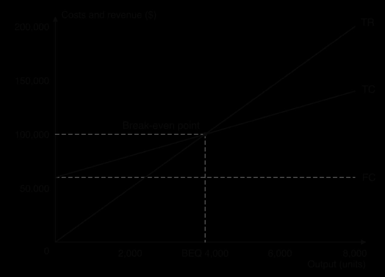
The chart shows that the total cost line starts at the fixed cost line, not at zero, because the business must pay its fixed costs even if it produces nothing. The total cost line rises at a slope equal to the variable cost per unit ($10 per bottle), and the total revenue line rises at a slope equal to the price ($25 per bottle). Because revenue rises faster than cost, the two lines must cross, and they cross at 4,000 bottles.
Once the lines are drawn, the chart shows the result at every level of output. To the left of the break-even point the total cost line is above the total revenue line: the vertical gap between them is the loss at that output. To the right of the break-even point the total revenue line is above the total cost line, and the vertical gap is the profit. The two regions between the lines are called the profit and loss areas.
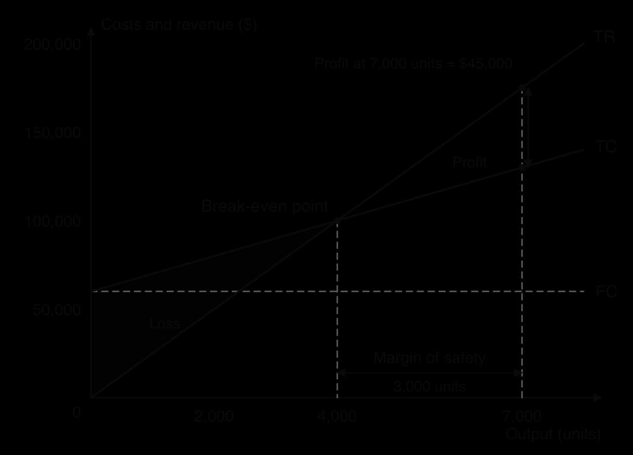
The profit at any output can be read from the chart by measuring the vertical distance between TR and TC at that output. At 7,000 bottles, TR is $175,000 and TC is $130,000, so the profit is $45,000. At 2,000 bottles, TR is $50,000 and TC is $80,000, so the loss is $30,000. The loss at zero output equals the fixed costs, $60,000, because the business has no revenue at all.
The profit area widens as output rises because each extra bottle adds the same $15 of contribution. This is why businesses with a high contribution per unit gain so much from extra sales once they pass the break-even point, and lose so much when sales fall below it.
Reading profit from a chart is quick but only as accurate as the drawing. The exact figure comes from either of two equivalent formulas.
The second formula is usually faster. A negative answer is a loss and is written in brackets in a financial table, for example ($30,000), or with a minus sign in a sentence.
The break-even quantity on its own does not show how close a business is to making a loss. The margin of safety measures how far current or forecast sales are above the break-even quantity, which is how much sales could fall before the business starts to make a loss.
AquaLoop forecasts sales of 7,000 bottles and breaks even at 4,000, so its margin of safety is 7,000 − 4,000 = 3,000 bottles. Sales could fall by 3,000 bottles before the business made a loss. On the break-even chart, the margin of safety is the horizontal distance between the break-even quantity and the forecast output, shown with a double-headed arrow.
The margin of safety can also be expressed in revenue, by multiplying it by the price: 3,000 × $25 = $75,000 of sales. Some businesses state it as a percentage of actual output, which makes it easier to compare businesses of different sizes.
A large margin of safety means the business can absorb a sizeable fall in sales and still cover its costs, so it is in a less risky position. A small margin of safety means that a modest fall in demand, a new competitor or a recession could push it into loss. If actual output is below the break-even quantity, the margin of safety is negative: a margin of safety of −500 units means the business is 500 units short of breaking even and is making a loss.
What counts as a “safe” margin depends on how stable demand is. A water utility with steady demand can operate safely with a small margin of safety. A fashion brand or a business selling luxury goods, whose sales can swing widely from year to year, needs a much larger one.
A tutor2u video works through the margin of safety on a chart and by calculation.
 YouTube
Most businesses do not aim simply to break even. Owners and managers set a target profit for the year, for example to pay back a loan, to fund new investment or to give shareholders a return. Break-even analysis can be extended to find the output that delivers that profit.
To make a target profit, the total contribution must cover the fixed costs and the target profit as well. So the fixed costs and the target profit are added together and divided by the contribution per unit. The result is the target profit output.
The formula is the break-even formula with the target profit added to the top. Break-even quantity is simply the target profit output when the target profit is zero.
Sometimes output is fixed, for example by the size of a factory, the number of seats in a theatre or a forecast of demand, and the question is what price would give the target profit. The target price answers it. At that price, the revenue from the given output covers the variable costs, the fixed costs and the target profit.
The formula works in two parts. The fraction is the contribution each unit must make for the given output to cover the fixed costs and the target profit. Adding the variable cost per unit turns that required contribution into a price. If the target profit is zero, the formula gives the break-even price: the lowest price at which the given output covers all costs.
Break-even data is often presented in words or in a table, and a complete chart is constructed from it with the key figures marked. The worked example follows the construction steps on a new set of figures and adds the margin of safety and the profit at the forecast output.
Break-even analysis is most useful when it is used to ask “what if?”. A change in price changes the slope of the total revenue line; a change in the variable cost per unit changes the slope of the total cost line; a change in fixed costs moves the fixed cost and total cost lines up or down. Each change moves the break-even point, the profit at a given output and the margin of safety. The effects can be shown by drawing the new line on the chart and by recalculating.
Change (all else equal) | Line that moves | Contribution per unit | Break-even quantity | Profit at a given output | Margin of safety |
|---|---|---|---|---|---|
Price rises | TR becomes steeper (pivots up from the origin) | Rises | Falls | Rises | Rises |
Price falls | TR becomes flatter | Falls | Rises | Falls | Falls |
Variable cost per unit rises | TC becomes steeper (pivots up from the FC level) | Falls | Rises | Falls | Falls |
Variable cost per unit falls | TC becomes flatter | Rises | Falls | Rises | Rises |
Fixed costs rise | FC and TC shift up in parallel | No change | Rises | Falls | Falls |
Fixed costs fall | FC and TC shift down in parallel | No change | Falls | Rises | Rises |
The table assumes that only one thing changes and, in particular, that the number of units sold stays the same. In reality a price change usually changes the quantity demanded as well, so the effect on profit has to be judged with care. The examples use AquaLoop’s original position as the starting point: price $25, variable cost $10, fixed costs $60,000, forecast output 7,000 bottles, break-even quantity 4,000, margin of safety 3,000 bottles and profit $45,000.
If AquaLoop raises its price from $25 to $30, each bottle brings in $5 more revenue but costs the same to make, so the contribution per unit rises from $15 to $20. The total revenue line still starts at the origin but becomes steeper, and it now crosses the unchanged total cost line sooner.
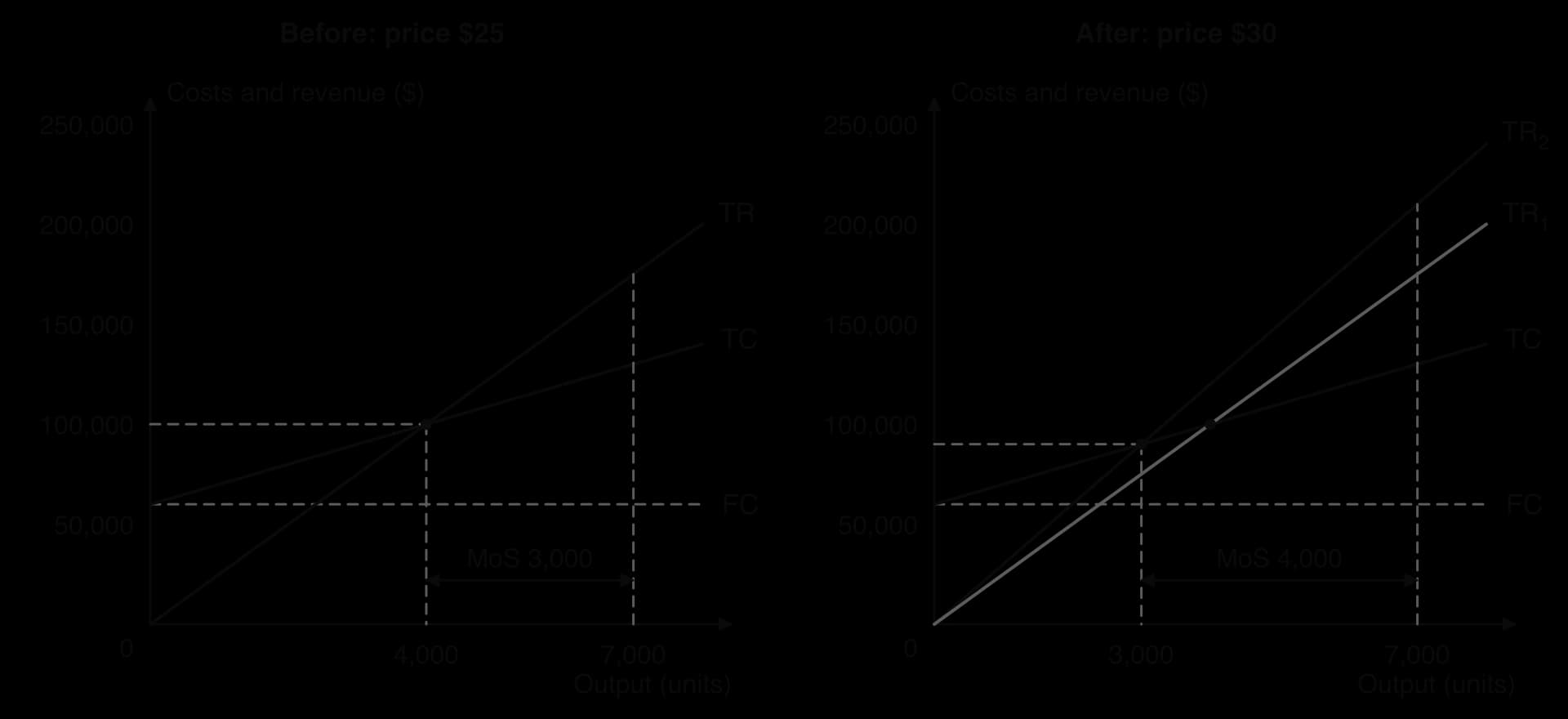
The recalculation confirms the chart. The new break-even quantity is $60,000 ÷ $20 = 3,000 bottles. If sales stay at 7,000 bottles, the margin of safety rises to 7,000 − 3,000 = 4,000 bottles and the profit to ($20 × 7,000) − $60,000 = $80,000.
The weakness of this calculation is the assumption that sales stay at 7,000. Higher prices usually reduce the quantity customers buy. At $30 AquaLoop needs to sell only 5,250 bottles to earn its original profit of $45,000 (($60,000 + $45,000) ÷ $20), so the price rise increases profit as long as sales fall by less than 1,750 bottles, or 25%. Whether they would depends on how loyal customers are, how many close substitutes exist and how competitors respond.
Costco shows how powerful a price rise can be when it adds almost nothing to variable costs. From 1 September 2024 the warehouse club raised its basic annual membership fee in the United States and Canada to $65 and its Executive membership from $120 to $130. Serving a member costs Costco little more after the rise than before, so almost the whole increase adds to contribution, as long as members renew.
Sources: Costco Wholesale Corporation, Form 10-K for the fiscal year ended 1 September 2024.
A price cut has the opposite effect. If AquaLoop cut its price to $20, its contribution per unit would fall to $10, the TR line would become flatter, and the break-even quantity would rise to $60,000 ÷ $10 = 6,000 bottles. At the forecast of 7,000 bottles, the margin of safety would shrink to 1,000 bottles and profit to ($10 × 7,000) − $60,000 = $10,000.
A business cuts its price only if it expects sales to rise enough to make up for the lower contribution per unit. To earn the original $45,000 profit at $20, AquaLoop would need to sell ($60,000 + $45,000) ÷ $10 = 10,500 bottles, which is more than its factory can make. This shows the risk of using price cuts to win sales when contribution per unit is small: the extra sales needed rise very quickly.
Variable costs rise when raw materials, energy or packaging become more expensive, or when piece-rate wages increase. If the cost of steel pushes AquaLoop’s variable cost from $10 to $13 per bottle, its contribution per unit falls from $15 to $12. The total cost line still starts at $60,000 but becomes steeper.
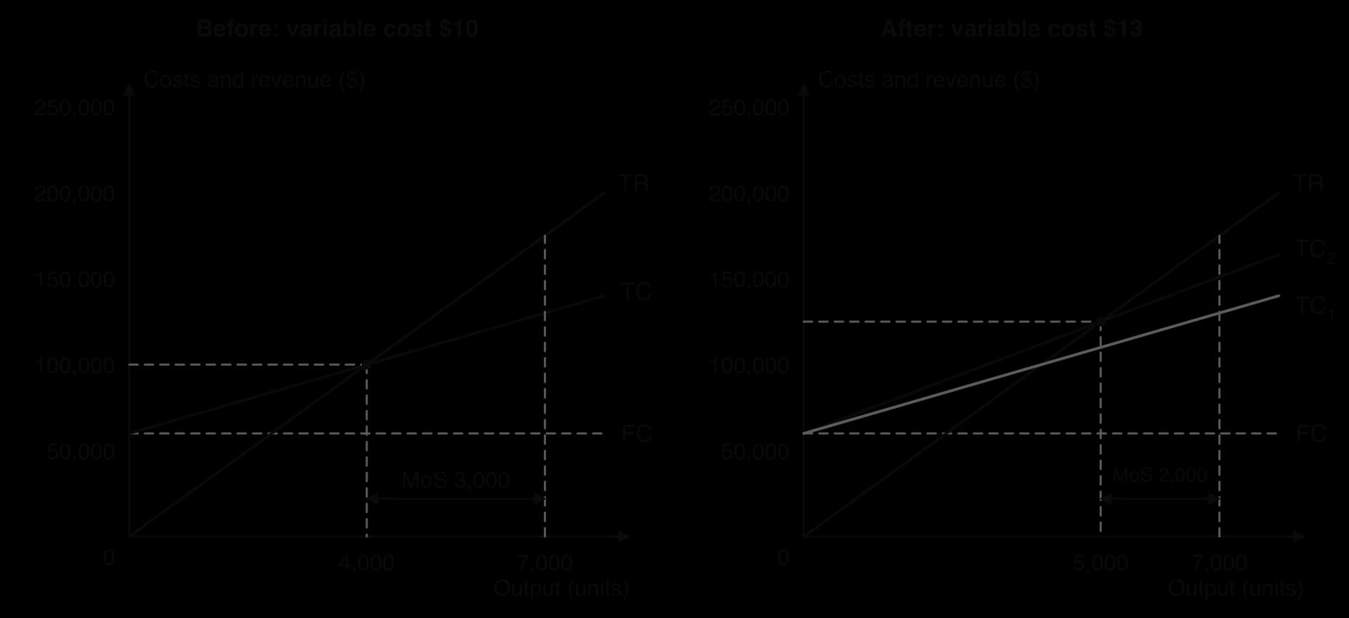
The new break-even quantity is $60,000 ÷ $12 = 5,000 bottles. At 7,000 bottles the margin of safety falls to 2,000 bottles and profit to ($12 × 7,000) − $60,000 = $24,000, little more than half of the original profit. A rise of 30% in the variable cost per unit has cut profit by 47%, because the whole rise comes out of contribution while fixed costs stay the same.
A business facing higher variable costs has three broad options: absorb the cost and accept lower profit, pass it on to customers through a higher price, or look for cheaper inputs. Passing the cost on restores the contribution per unit but risks losing sales; cheaper inputs may lower quality or raise ethical concerns about suppliers.
Fixed costs rise when rent is increased, when the business takes on more salaried staff or when it invests in new equipment that must be leased or paid for with a loan. If AquaLoop’s rent rises so that its fixed costs go up from $60,000 to $75,000, the contribution per unit is unchanged at $15, but more units are needed to cover the higher fixed costs.
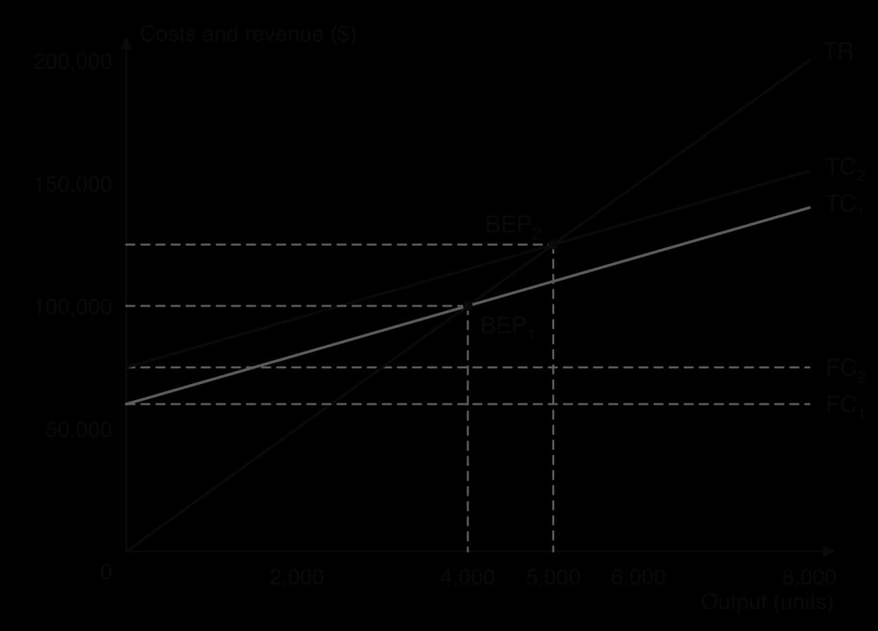
The new break-even quantity is $75,000 ÷ $15 = 5,000 bottles. At 7,000 bottles the margin of safety falls to 2,000 bottles and profit to ($15 × 7,000) − $75,000 = $30,000. Profit falls by exactly the rise in fixed costs, $15,000, because fixed costs are subtracted in full whatever the level of output.
The two cost rises give the same break-even quantity in this example (5,000 bottles) but affect the business differently as output changes. A rise in fixed costs moves the whole TC line up by the same amount, so it costs the business $15,000 at any output. A rise in variable cost per unit makes TC steeper, so it costs more the more the business sells: $21,000 at 7,000 bottles, but $24,000 at 8,000.
Real decisions often involve several changes together. A price rise may be expected to reduce sales; a new machine may raise fixed costs but lower the variable cost per unit. The method is the same: recalculate the contribution per unit, then the break-even quantity, the margin of safety and the profit at the expected output, and compare the results with the original position.
The example shows a general trade-off. Replacing variable costs with fixed costs, for example by automating, raises profit at high output but makes the business more vulnerable when sales fall, because the fixed costs must be paid whatever happens. Businesses with stable, high demand can benefit from this structure; those with uncertain demand often prefer to keep costs variable, for example through outsourcing.
Break-even analysis is used by businesses of every size because it turns a few figures into clear answers to practical questions.
Starting a business. A start-up includes a break-even calculation in its business plan to show banks and investors how many units it must sell, and how quickly, before it stops losing money.
Pricing. Managers test how a price change would affect the break-even quantity and profit before they make it, and find the lowest price that still covers costs at a given output.
Cost control. The analysis shows how much a rise in rent or in raw material prices would cost, and how many extra units would be needed to make up for it.
Investment and expansion. It shows whether a new product, branch or machine is likely to reach break-even at the expected level of demand, alongside investment appraisal.
Setting targets. Target profit output and target price turn a profit objective into a sales target or a price for the sales and marketing teams.
The tool also connects to the four key concepts of the course, which are summarised in the table.
Key concept | How it links to break-even analysis |
|---|---|
Change | Every change in price, variable cost or fixed cost moves the break-even point; regular recalculation shows how a business must adapt to rising costs or new competition. |
Creativity | Creative solutions can lower the break-even point: new revenue streams, a premium version of a product that raises contribution per unit, or new processes that cut variable costs. |
Ethics | Pressure to break even can lead to unethical cost cutting, such as paying suppliers below a fair price or cutting safety spending, which lowers costs on paper but harms stakeholders. |
Sustainability | Sustainable materials and fair wages often raise variable costs and the break-even quantity in the short run, but can strengthen the brand and reduce risk in the long run. |
Break-even analysis is simple because of its assumptions, and each assumption is also a limitation. Managers who use it need to know where the answer may be misleading.
The model draws TR and TC as straight lines, which assumes that every unit sells at the same price and costs the same to make. In practice businesses offer discounts for bulk orders, so the average price falls as sales rise and the TR line bends downwards. Costs are not constant either: economies of scale can lower the variable cost per unit at high output, while overtime pay and machine breakdowns can raise it when a factory runs near its limit.
Break-even analysis assumes that everything produced is sold, with no unsold stock. Many businesses produce ahead of demand, and goods that are not sold, or are sold later at a discount, do not bring in the revenue the chart assumes. Perishable products, such as fresh food or fashion items, are especially exposed to this.
The basic model works for one product with one price. Most businesses sell many products with different prices and variable costs, and share fixed costs, such as rent and managers’ salaries, among them. Break-even analysis can be applied to the whole business only by assuming a fixed sales mix, or to each product only by dividing up the fixed costs, which involves judgment.
A break-even chart shows the position at one moment in time, based on one set of costs and prices. Real costs and prices change frequently, as the airline industry’s fuel bills show, so the chart quickly becomes out of date and must be redrawn whenever conditions change.
Fixed costs are fixed only within a range of output. To produce beyond the capacity of its factory, a business needs extra premises, machines or managers, so its fixed costs rise in a step. AquaLoop could sell more than 8,000 bottles only by adding a new production line, which would create a new, higher fixed cost line and a new break-even point.
A factory, a machine or a manager can handle only a certain volume of work. Up to that volume, fixed costs stay the same. To go beyond it, the business must add a whole new unit of capacity, such as a second production line, even if it needs only a little extra output. Total fixed costs therefore jump at that point and stay level again until the next limit. These are sometimes called stepped fixed costs.
For break-even analysis, this means a chart is valid only within one “step”. A business planning a large expansion needs a new chart with the higher fixed costs, and it may find that its break-even quantity rises sharply just after it expands.
Break-even analysis deals only with numbers. It says nothing about how customers would react to a price rise, how competitors would respond, whether employees would accept a new machine, what a cost cut would do to quality or the brand, or whether a decision is ethical. These factors often decide whether a plan succeeds.
The results are only as accurate as the forecasts of price, cost and sales behind them. A new business has no sales history and may be optimistic, and costs such as energy can change sharply. Classifying costs as fixed or variable also involves judgment, so two managers can produce different break-even points for the same business.
Strengths | Limitations |
|---|---|
Quick and cheap to calculate from a few figures. | Assumes straight-line costs and revenue, which ignores discounts and economies of scale. |
The chart shows profit or loss at every output in one picture, which helps managers, banks and investors understand a plan. | Assumes all output is sold at one price. |
Shows the margin of safety, a simple measure of risk. | Hard to apply to a business with many products and shared fixed costs. |
Easy to test “what if?” changes in price and cost. | Static: needs redrawing every time a cost or price changes. |
Turns profit objectives into sales targets and target prices. | Ignores qualitative factors such as customer reactions, competition and ethics. |
A standard part of a business plan for a start-up seeking finance. | Only as reliable as the forecasts of costs and sales behind it. |
How useful break-even analysis is depends on the business and the decision. It is most useful for a single-product business with stable prices and costs, such as a small manufacturer or an event organiser, and for quick decisions where a rough answer is enough, such as whether a price cut could pay for itself. It is least useful for a business with many products, frequent price changes or volatile costs, and for long-term strategic decisions, where qualitative factors dominate.
Break-even analysis is therefore best treated as a starting point. It identifies how many units a plan needs and how much risk it carries, but its answer should be checked against market research on the likely level of sales, combined with other tools such as cash flow forecasts and investment appraisal, and weighed against the qualitative factors before a decision is made.
Airlines are one of the clearest real examples of break-even analysis at work. An airline’s “units” are seats, and the share of the seats it sells is called the load factor. Airlines and their industry body, the International Air Transport Association (IATA), report the load factor an airline must achieve to cover its costs at the fares it is charging: the break-even load factor. It is the break-even quantity expressed as a percentage of capacity.
The industry has a cost structure that makes break-even critical. Once a flight is scheduled, most of its cost is fixed for that flight: the aircraft (whether owned or leased), the crew’s pay, most of the fuel, maintenance, and airport and air traffic control charges. An extra passenger adds only a small variable cost, such as a meal, a little extra fuel and the booking fee. The contribution from each extra seat sold is therefore high, and profit is very sensitive to the load factor.
Whether fuel counts as a fixed or a variable cost depends on the decision. Once a route is planned, fuel is largely fixed per flight. Across a year, however, an airline that flies more flights buys more fuel, so at industry level fuel behaves like a variable cost.
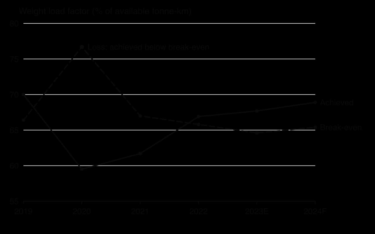
IATA’s industry statistics compare the break-even load factor with the load factor airlines actually achieved. The difference works like a margin of safety: it shows how many percentage points of capacity airlines could have lost before falling into an operating loss. The chart and table use IATA’s weight load factor, which measures passengers and cargo together as a share of the available capacity in tonne-kilometres.
Year | Break-even weight load factor (%) | Achieved weight load factor (%) | Difference (percentage points) | Industry operating profit ($ billion) |
|---|---|---|---|---|
2019 | 66.4 | 70.0 | 3.6 | 43.2 |
2020 | 76.7 | 59.5 | (17.2) | (110.8) |
2021 | 67.0 | 61.7 | (5.3) | (44.2) |
2022 | 65.8 | 66.9 | 1.1 | 11.9 |
2023 (estimate) | 64.6 | 67.7 | 3.1 | 40.7 |
2024 (forecast) | 65.4 | 68.9 | 3.5 | 49.3 |
The figures follow the logic of a break-even chart closely. In 2019 airlines operated 3.6 points above break-even and made an operating profit of $43.2 billion. When the COVID-19 pandemic closed borders in 2020, the achieved load factor collapsed to 59.5% while the break-even load factor jumped to 76.7%, because fixed costs such as aircraft and staff continued while revenue disappeared. The margin of safety became a deficit of 17.2 points, and the industry’s operating loss was $110.8 billion. As traffic returned in 2022, the achieved load factor rose just above break-even and the industry returned to a small operating profit.
The data also shows that the break-even point itself moves. Its level depends on fares and costs, which change from year to year. The break-even load factor fell from 67.0% in 2021 to 64.6% in 2023 partly because fares rose: passenger yields (average revenue per passenger-kilometre) increased by 9.5% in 2022 and 6.2% in 2023, which in break-even terms is a steeper TR line. Fuel worked in the other direction, rising from 19% of airline expenses in 2021 to 32% in 2023.
IATA’s June 2026 outlook shows a sudden change in variable costs. After the Strait of Hormuz was effectively closed to commercial shipping on 28 February 2026, IATA reported that the price of jet fuel had roughly doubled. It forecast an average jet fuel price of $152 a barrel for 2026, against $90 in 2025, with fuel rising from 25.4% to 31.4% of airline expenses. In break-even terms, the TC line became much steeper.
Airlines responded as break-even analysis predicts: they raised fares to restore contribution per passenger. IATA forecast a 7.0% rise in passenger ticket yields for 2026 and record load factors of 84.0% of seats, helped by a shortage of new aircraft. Even so, the higher fares did not fully offset the fuel bill, and IATA forecast that the industry’s net profit margin would halve.
Global airline industry | 2025 (estimate) | 2026 (forecast) |
|---|---|---|
Jet fuel price ($ per barrel) | 90 | 152 |
Fuel as a share of expenses (%) | 25.4 | 31.4 |
Passenger ticket yield (% change on the year before) | 0.5 | 7.0 |
Passenger load factor (% of seats sold) | 83.5 | 84.0 |
Net profit margin (%) | 4.2 | 2.0 |
Net profit per departing passenger ($) | 9.10 | 4.50 |
Source: IATA, Global Outlook for Air Transport, June 2026.
The case also shows the limits of the tool. Industry averages hide large differences between low-cost and full-service airlines and between regions. Fares are not one price but many, set by yield management, so the TR line is not really straight. And the break-even load factor depends on forecasts of fuel prices and fares that can change within weeks, as the events of 2026 showed. Airlines therefore recalculate break-even constantly and combine it with fuel hedging, capacity planning and pricing decisions.
Sources: IATA, Industry Statistics Fact Sheet (December 2023); IATA, Global Outlook for Air Transport (June 2026).
Explain why an airline’s profit is very sensitive to its load factor, using the terms contribution and fixed costs.
Using the table, explain how the margin of safety changed between 2019 and 2020, and why.
Analyse how the 2026 rise in jet fuel prices and the rise in fares affected the break-even load factor, using a sketch of a break-even chart.
Break-even analysis appears mostly in Paper 2, where questions ask for calculations and charts from data, and sometimes in Paper 1 as a short calculation. Typical questions ask you to define a term, calculate contribution, the break-even quantity, the margin of safety, the target profit output or the target price, construct a chart, show the effect of a change, and then evaluate a decision using the results.
Charts that show a change are marked on the new line as well as the original ones.
The questions are based on a short case.
Kibo Cycles assembles electric bicycles in a small workshop in Nairobi. Each bicycle sells for $1,200 and has a variable cost of $700 (motor, battery, frame and assembly labour). Monthly fixed costs are $40,000. The workshop can assemble up to 150 bicycles a month, and Kibo expects to sell 110 a month. The owner is considering cutting the price to $1,100 to win orders from delivery companies, which she expects would raise sales to 130 a month (hypothetical data).
Calculation questions often come in a sequence, with later parts using earlier answers.
A construction question checks that the chart is accurate and complete.
Target questions combine the formulas with the capacity of the business.
Questions on the effects of a change ask for both the new figures and an explanation.
The extended response asks for a judgment that uses the calculations as evidence and goes beyond them.
Contribution per unit is price minus variable cost per unit; total contribution is contribution per unit × quantity, or TR − TVC; profit is total contribution minus fixed costs.
The break-even quantity, where TR = TC, is fixed costs ÷ contribution per unit, rounded up to a whole unit.
A break-even chart shows FC (horizontal), TC (starting at FC) and TR (from the origin); the break-even point is where TR crosses TC, with the loss area to its left and the profit area to its right.
The margin of safety is actual output minus the break-even quantity: how far sales can fall before a loss.
Target profit output = (fixed costs + target profit) ÷ contribution per unit; target price = (fixed costs + target profit) ÷ output + variable cost per unit.
A price rise or a fall in costs lowers the break-even quantity and raises the margin of safety and profit; a price cut or a rise in costs does the opposite.
Break-even analysis is quick and clear but assumes linear costs and revenue, one product and that all output is sold, and it ignores qualitative factors and cash flow.
I can distinguish between contribution per unit and total contribution, and calculate both.
I can calculate the break-even quantity and break-even revenue, rounding correctly.
I can calculate profit or loss at any level of output by two methods.
I can construct a fully labelled break-even chart from data, step by step.
I can show the break-even point, the profit and loss areas and the margin of safety on a chart.
I can calculate the margin of safety, the target profit output and the target price.
I can show and calculate the effects of changes in price, variable costs and fixed costs.
I can evaluate break-even analysis as a decision-making tool, using a real case.
Using your answers to (a), calculate the break-even quantity under each pricing strategy (show all your working).
3 marks
Award [1] for correct working, [1] for each correct answer, up to [3]. Accept 466 666.67 or 466 667 cartons (rounded up). Accept OFR from (a).
Calculate the forecast profit for the first year under each pricing strategy (show all your working).
3 marks
Premium: (400 000 × 2.80) − 700 000 = 1 120 000 − 700 000 = CAD 420 000
Penetration: (750 000 × 1.50) − 700 000 = 1 125 000 − 700 000 = CAD 425 000
Award [1] for correct working and [1] for each correct answer, up to [3]. Award a maximum of [2] if the currency is missing. Accept OFR from (a).
Calculate the margin of safety under the premium pricing strategy.
2 marks
400 000 − 250 000 = 150 000 cartons
Award [1] for working and [1] for the correct answer with units. Accept OFR from (b).
Using your answers to (a) to (d) and other information, recommend which pricing strategy POC should use for its new oat drink.
10 marks
Premium pricing (CAD 4.50):
Forecast profit CAD 420 000, almost identical to penetration, but on far fewer cartons; break-even at 250 000 cartons, so sales could fall by 150 000 (37.5 %) before POC makes a loss.
Uses only half the 800 000 capacity, leaving room for growth; fits a differentiated position on local sourcing.
Lower working capital and fewer supply problems with local farmers.
However, the price is CAD 0.70 above the international brands, so the 400 000 forecast relies on customers valuing local sourcing; coffee shops are price-conscious buyers.
Penetration pricing (CAD 3.20):
Forecast profit CAD 425 000 and higher market share; undercuts the international brands by CAD 0.60, which may win coffee-shop contracts; larger volume may bring economies of scale and supplier discounts later.
However, break-even is 466 667 cartons and the margin of safety only 283 333 cartons; forecast sales of 750 000 are close to full capacity (93.75 %), leaving no room to meet extra demand; the low contribution (CAD 1.50) makes profit very sensitive to forecast errors; the two international brands may cut prices in response; raising prices later may be difficult.
Possible recommendation: premium pricing gives nearly the same profit with less risk and supports the brand, but penetration may build share in a growing market. Any substantiated recommendation can earn full marks.
Limitations: the sales forecasts are estimates from POC’s own team; variable cost is assumed constant; no information on competitors’ reactions or longer-term profits.
Marks should be allocated according to the markbands below.
Additional guidance:
If only one option is discussed, even with balance, award a maximum of [5]; one option, one-sided, a maximum of [3].
A response that makes no use of the data or case details the question refers to cannot be awarded more than [4].
A response with no conclusion or judgement will typically not be awarded more than [6].
Markbands (10-mark extended response, Papers 1 and 2)
Marks | Level descriptor |
|---|---|
0 | The response does not reach the standard described below. |
1–2 | Little understanding of what the question demands. Business management tools and theories are barely used, or are irrelevant or inaccurate. Little or no reference to the stimulus material. No arguments are made. |
3–4 | Some understanding of what the question demands. Some use of tools and theories, but mostly inaccurate or not relevant. Use of the stimulus is superficial, often no more than the name of the organisation or person. Arguments are mostly unsubstantiated. |
5–6 | Understands what the question demands but addresses it only partially. Some relevant, accurate use of tools and theories. Some relevant use of the stimulus beyond names, but it does not effectively support the argument. Arguments are substantiated but mostly one-sided. |
7–8 | Mostly addresses what the question demands. Mostly relevant, accurate use of tools and theories. The stimulus generally supports the argument, with some lapses in clarity or relevance. Arguments are substantiated and show some balance. |
9–10 | Clear focus on what the question demands. Relevant, accurate use of tools and theories. Relevant stimulus material is integrated effectively to support the argument. Arguments are substantiated and balanced, and the limitations of the case or stimulus material are explained. |
A response with no judgement or conclusion is unlikely to reach the top band of a discuss, evaluate, examine or recommend question.
Taa Yetu Solar
Taa Yetu Solar (TYS) is a private limited company in Kisumu, Kenya. It assembles home solar kits (a panel, a battery, wiring and three lights) for households that are not connected to the electricity grid. TYS sells each kit for KES 18 000 and currently assembles and sells 600 kits per month. Its monthly costs are shown in Table 1.
Table 1: TYS’s monthly costs
Cost | Amount (KES) |
|---|---|
Rent of assembly workshop | 180 000 per month |
Salaries of four administrative and sales staff | 360 000 per month |
Insurance | 40 000 per month |
Solar panel | 6 500 per kit |
Battery | 4 200 per kit |
Wiring, lights and packaging | 800 per kit |
Delivery to the customer | 500 per kit |
Define the term fixed costs.
2 marks
Using Table 1, calculate TYS’s total costs per month (show all your working).
2 marks
Calculate the average cost of a kit (show all your working).
2 marks
Calculate TYS’s monthly profit (show all your working).
2 marks
TYS plans to raise output to 900 kits per month without any change in its fixed costs. Explain, with a supporting calculation, the effect of this on TYS’s average cost per kit.
4 marks
Shine Bay Car Wash
Shine Bay Car Wash (Shine Bay) is a partnership owned by Sibusiso Zungu and Priya Naidoo in Durban, South Africa. It charges R120 for a standard wash. Attendants are paid R20 for every car they wash, in addition to a basic monthly salary paid only to the manager. In March, Shine Bay washed 1 400 cars.
Table 1: Shine Bay’s costs
Cost | Amount (R) |
|---|---|
Lease of site | 28 000 per month |
Manager’s salary | 22 000 per month |
Lease of washing equipment | 9 500 per month |
Insurance | 3 500 per month |
Water | 12 per car |
Cleaning chemicals | 9 per car |
Electricity | 4 per car |
Attendants’ pay | 20 per car |
Using Table 1, calculate Shine Bay’s total costs for March (show all your working).
2 marks
Calculate the average cost of a car wash in March (show all your working).
2 marks
Calculate Shine Bay’s profit for March (show all your working).
2 marks
Because of a drought, the city council has doubled water tariffs, so water now costs Shine Bay R24 per car. Assuming Shine Bay still washes 1 400 cars a month at R120, explain the effect of this change on Shine Bay’s costs and profit. Support your answer with calculations.
4 marks