Notes on 4.3 Sales forecasting
Learning objectives
Define sales forecasting and explain why businesses forecast their sales.
Distinguish between qualitative and quantitative methods of sales forecasting.
Explain the four components of a time series: trend, seasonal, cyclical and random variation.
Calculate three-period moving averages and centred four-period moving averages.
Calculate seasonal variations and use them with an extrapolated trend to forecast sales.
Explain how extrapolation and simple linear regression are used to forecast sales.
Evaluate the benefits and limitations of sales forecasting for a business.
Introduction
Every plan a business makes depends on how much it expects to sell. A sales forecast turns past sales, market information and managers’ judgment into an estimate of future sales, and that estimate then drives decisions on production, stock, staffing, cash and finance. A good forecast lets a business prepare for demand before it arrives; a poor one leaves it with empty shelves or a warehouse full of unsold goods.
Forecasting is a response to change: markets move with consumer tastes, technology, competition and the state of the economy, and a forecast is the business’s best attempt to anticipate those movements. It also raises questions of ethics and sustainability, because forecasts presented to investors must be honest, and forecasts that overestimate demand lead to overproduction and waste.
What a sales forecast is
Sales forecasting is the process of predicting the quantity or value of sales a business expects to make over a future period, such as the next month, quarter or year. The forecast can be expressed in units (12,000 bicycles), in sales revenue ($3.6 million) or as a share of the market. Most businesses forecast sales for each product, each region and each period separately, because each part of the business needs a different level of detail.
A forecast is the starting point for most other plans. The marketing plan sets marketing objectives and budgets from it; the operations department uses it to schedule output and order materials; the finance department turns it into a cash flow forecast and a sales revenue budget; and human resources uses it for workforce planning. If the sales forecast is wrong, every plan built on it is wrong too.
Forecasting horizons
The period a forecast covers is its horizon. Short-term forecasts are more accurate because fewer things can change in a few weeks than in five years, but long-term forecasts are still needed for large investments such as a new factory, whose returns depend on sales many years ahead.
Horizon | Typical period | Used for | Main methods |
|---|---|---|---|
Short term | Up to 1 year (weeks, months, quarters) | Ordering stock, scheduling production and shifts, monthly cash flow forecasts | Moving averages, seasonal variation, sales force estimates |
Medium term | 1–3 years | Annual budgets, marketing plans, recruitment, product launches | Trend extrapolation, regression, market research |
Long term | 3 years or more | Investment in capacity, new markets, strategic plans | Expert opinion, the Delphi method, scenarios based on economic forecasts |
Methods of sales forecasting
Forecasting methods fall into two groups. Qualitative methods rely on the judgment and experience of people who know the market. Quantitative methods use numerical data, usually past sales, and mathematical techniques to find patterns that can be projected forward. Most businesses use both and compare the results.
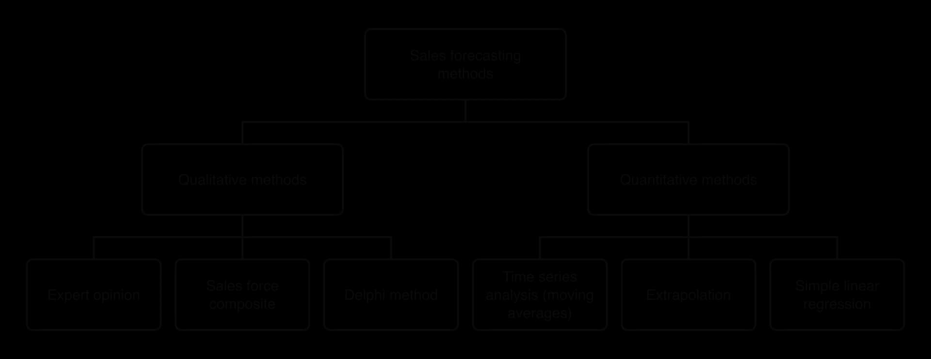
Qualitative forecasting
Qualitative forecasting is used when there is little or no reliable past data (a new product, a new market) or when the future is likely to differ from the past (a new competitor, a change in regulation, a recession). It produces numbers too, but those numbers come from informed opinion rather than from a calculation.
Expert opinion
Managers may ask people with specialist knowledge for their view of future demand: industry analysts, economists, consultants, trade associations or experienced senior staff. Expert opinion is quick and can take account of events that past data cannot show, such as a planned change in the law. Its weakness is that experts can be wrong, can disagree with one another and can be biased by their own interests.
Sales force composite
In a sales force composite, each salesperson estimates how much they expect to sell to their own customers or in their own territory over the coming period. The estimates are added together, and then adjusted by sales managers, to give a forecast for the whole business. The method is common in business-to-business markets, where salespeople deal with a small number of large customers and know their plans well.
The method uses the knowledge of the people closest to customers, but it has a built-in bias. If salespeople are paid commission or judged against targets set from their own forecasts, they have an incentive to forecast low, so that the targets are easy to beat. Optimistic salespeople may forecast too high. Managers therefore compare the composite with past accuracy and with quantitative forecasts.
The Delphi method
The Delphi method was developed at the RAND Corporation in the United States in the 1950s to forecast developments in technology. It gathers the opinions of a panel of experts in several rounds, anonymously, so that the final forecast reflects the group’s reasoning rather than the views of its most senior or most confident member.
A coordinator chooses a panel of experts and sends each of them a questionnaire (for example, “What will total sales of electric scooters in India be in 2030?”).
The experts answer individually and anonymously, giving reasons.
The coordinator summarises the answers (the range, the median forecast and the main reasons) and sends the summary back to the panel.
Each expert reconsiders their forecast in the light of the others’ reasoning and answers again.
The rounds continue until the answers converge; the final forecast is usually the median of the last round.
Anonymity reduces the pressure to agree with a dominant person, and the rounds let experts learn from one another. The method is slow and costly, however, and the result depends on the choice of experts. It suits long-term forecasts in new or uncertain markets, where there is no useful past data.
Market research as a basis for forecasts
A business can also ask customers directly. Surveys of buying intentions, test marketing and focus groups are forms of market research that produce estimates of demand for a new product. These estimates are often too high, because people say they will buy more than they actually do, so firms usually scale them down using experience from earlier launches.
Quantitative forecasting
Quantitative methods start from numerical data. The most common is time series analysis: studying sales recorded at regular intervals (each month, quarter or year) to identify the underlying trend and the regular patterns around it, then projecting them forward. A second approach looks for a relationship between sales and another variable, such as advertising spending or household income, and uses that relationship to predict sales; this is simple linear regression, which uses a scatter diagram and a line of best fit.
Qualitative methods | Quantitative methods | |
|---|---|---|
Based on | Judgment, experience and opinion | Past numerical data and statistical techniques |
Examples | Expert opinion, sales force composite, Delphi method, surveys of buying intentions | Moving averages, seasonal variation, extrapolation, simple linear regression |
Best when | There is little past data, or the future is likely to differ from the past | There is plenty of reliable past data and the market is fairly stable |
Main strength | Can allow for new events, products and competitors | Objective and repeatable; the reasoning can be checked |
Main weakness | Open to bias and hard to check | Assumes past patterns will continue |
Time series analysis
A time series is a set of observations of one variable, such as sales revenue, recorded at regular intervals over time. Time series analysis breaks the series into its components so that each can be measured and projected. Actual sales in any period are treated as the combination of four components: the trend, seasonal variation, cyclical variation and random variation.
Trend
The trend is the long-run direction in which the data move once short-term ups and downs are removed: rising, falling or flat. Sales of a product in the growth stage of its life cycle show a rising trend; sales of a product in decline show a falling one. The trend is the most important component for medium- and long-term forecasts.
Seasonal variation
Seasonal variation is a regular, repeated pattern within a year. Ice cream and sun cream sell more in summer, heating oil and winter coats in winter, toys and electronics before the end-of-year holidays. Seasonal patterns can also follow the school year, religious festivals (Diwali, Ramadan, Lunar New Year) or the days of the week, as in restaurants that are busiest at weekends.
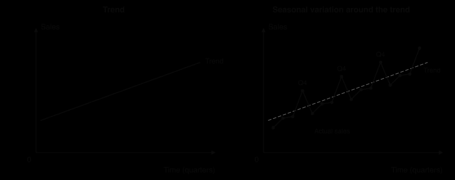
In the right-hand panel the seasonal pattern is the gap between actual sales and the trend in each quarter. Because the pattern repeats, it can be measured from past years and added to a forecast of the trend. US online retailers show this pattern clearly: e-commerce sales in the fourth quarter, which includes the end-of-year shopping season, are well above sales in the quarters on either side every year.
Cyclical variation
Cyclical variation is a longer wave of rises and falls linked to the business cycle of the whole economy: periods of boom, when incomes and spending rise, followed by recession, when they fall. A cycle typically lasts several years and is much less regular than a seasonal pattern. Sellers of cars, houses, furniture and holidays are strongly affected, because customers postpone these purchases when incomes are uncertain.
US sales of new cars and light trucks show the effect of a recession. They averaged about 17.5 million a year (at an annual rate) in 2005, fell to about 10.6 million in 2009 during the global financial crisis, and did not return to their earlier level until 2015.
Sources: US Bureau of Economic Analysis, Total Vehicle Sales (series TOTALSA), via FRED, retrieved October 2026; annual averages calculated from monthly data.
Random variation
Random variation is the part of the data that has no pattern: sudden, one-off changes caused by unpredictable events such as extreme weather, a fire at a supplier, a strike, a product recall or a viral social media post. In March 2021 the container ship Ever Given blocked the Suez Canal for six days, delaying goods for retailers across Europe; no past sales data could have predicted it.
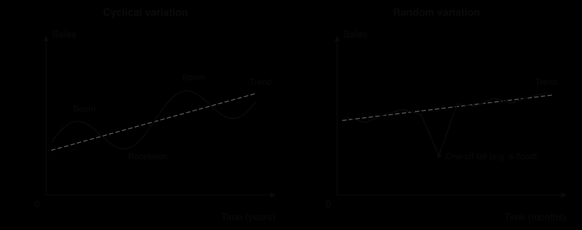
Random variation cannot be forecast, but it can be planned for. Businesses keep buffer stock, spread their suppliers and prepare a contingency plan so that one-off events do less damage.
 YouTube
Moving averages
To measure the trend, the seasonal and random ups and downs must be smoothed out. A moving average does this by replacing each value with the average of a group of consecutive values, then moving the group forward one period at a time. Each average contains one high season and one low season, or a full cycle of the pattern, so the peaks and troughs cancel out and the trend remains.
The number of periods in each average should match the length of the repeating pattern. Monthly data with a three-month pattern use a three-period moving average; quarterly data with a pattern that repeats every year use a four-period (four-quarter) moving average; daily data for a shop open seven days a week use a seven-day average.
Three-period moving averages
With an odd number of periods, each moving average belongs to the middle period of its group. The average of January, February and March is plotted against February; the average of February, March and April against March; and so on. The first and last periods have no moving average, because there are not enough values on both sides of them.
Four-period moving averages and centring
Quarterly data need a four-quarter moving average, so that each average contains one of each quarter. With an even number of periods, however, the middle of each group falls between two periods: the average of Q1 to Q4 belongs halfway between Q2 and Q3. To give each quarter its own trend value, the moving averages are centred by averaging each pair of neighbouring four-quarter averages.
The centred moving average for Q3 is the average of the four-quarter average for Q1–Q4 and the one for Q2–Q1 of the next year. In effect it is a weighted average of five quarters, with the two end quarters counted at half weight, so it still contains exactly one of each season.
The method is easiest to follow on real data. The table gives eight quarters of US retail e-commerce sales.
Quarter | Q1 2023 | Q2 2023 | Q3 2023 | Q4 2023 | Q1 2024 | Q2 2024 | Q3 2024 | Q4 2024 |
|---|---|---|---|---|---|---|---|---|
Sales ($bn) | 243.6 | 260.9 | 264.7 | 317.9 | 261.1 | 278.3 | 284.8 | 345.9 |
Sources: US Census Bureau, Quarterly Retail E-Commerce Sales, not seasonally adjusted, via FRED (series ECOMNSA), retrieved October 2026; rounded to $0.1 billion.
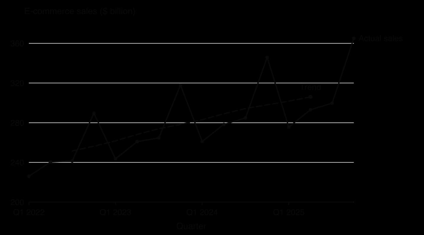
Repeating the calculation for every quarter from 2022 to 2025 gives the trend line in the chart. The actual series has a sharp peak every fourth quarter, while the centred moving average rises steadily from about $252 billion in Q3 2022 to about $306 billion in Q2 2025. The first two and last two quarters have no centred average, because there are not enough quarters on both sides of them.
Seasonal variation and forecasting
Once the trend is known, the seasonal pattern can be measured. For each period with a trend value, the seasonal variation is the difference between the actual figure and the trend. A positive figure means sales were above the trend in that period; a negative figure means they were below it.
A single year’s seasonal variation also contains random variation, so the variations for the same quarter in several years are averaged. The average seasonal variation for each quarter is the best estimate of how far that quarter normally sits above or below the trend.
Why do the average seasonal variations not add up to zero?
In a perfect additive model the four average seasonal variations would sum to zero, because over a year the ups and downs cancel out. Here they sum to −1.78. Some textbooks adjust each figure by a quarter of the difference so they total zero; the adjustment makes little difference to the forecast.
The table also shows that the Q4 variation grows each year (+33, +40, +48) as total sales grow. When the seasonal swing is a roughly constant percentage of sales rather than a constant amount, an additive model underestimates the swing in later years. Statisticians then use a multiplicative model, in which each season is expressed as a percentage of the trend.
Extrapolating the trend
To forecast, the trend is projected beyond the last known value. This is extrapolation: extending a pattern found in past data into a period for which there are no data yet. The trend can be extended by drawing a line of best fit through the plotted moving averages and continuing it, or by calculating the average change in the trend per period and adding it on.
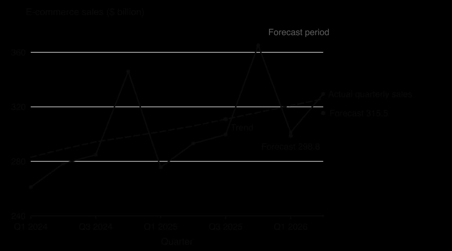
The chart shows both the strength and the weakness of the method. Where the market behaves as it did in the past, a moving-average forecast is cheap and accurate. Where growth speeds up or slows down, the forecast lags behind, because the trend is calculated from past periods only.
Simple linear regression as a forecasting method
A second quantitative method forecasts sales from their relationship with another variable. If past data show that a retailer’s sales rise in line with household income, or that a firm’s sales rise with its advertising spending, the relationship can be plotted on a scatter diagram, summarised by a line of best fit and used to predict sales for a given value of the other variable. This is simple linear regression.
Regression can also be used on a time series by treating time itself as the independent variable, so that the line of best fit through past sales becomes the trend line. Its reliability depends on the strength of the correlation between the two variables and on how far beyond the past data the forecast reaches, since extrapolation assumes the relationship holds outside the range observed.
Benefits of sales forecasting
A forecast is useful because it lets every part of the business prepare for future demand rather than react to it. The benefits are closely linked: better planning in one function usually helps the others.
Area | How the forecast is used | Benefit |
|---|---|---|
Operations | Scheduling production, ordering materials, setting stock levels, planning capacity | Fewer stock-outs and less excess stock; higher capacity utilisation; less waste |
Finance | Sales revenue budgets, cash flow forecasts, investment appraisal | Cash shortages are spotted early and an overdraft can be arranged in advance |
Human resources | Workforce planning: recruiting seasonal staff, training, overtime | The right number of workers with the right skills at the right time |
Marketing | Setting marketing objectives, timing promotions, allocating the marketing budget | Promotions can be timed to lift sales in weak periods |
Whole business | Business plans and loan applications | Banks and investors are more willing to provide finance |
Planning production and stock
A manufacturer that knows sales will peak in the fourth quarter can build up output and stock during the third quarter, order materials in good time and avoid paying for overtime or emergency deliveries at the peak. Accurate forecasts are especially important for businesses that use just-in-time production, which holds very little stock, and for perishable products such as fresh food, where unsold stock is thrown away.
Planning cash flow and budgets
Sales are the main source of cash inflows, so the sales forecast is the first line of the cash flow forecast. A business with seasonal sales may receive most of its cash in a few months while paying wages and rent every month; the forecast shows when a cash shortage is likely, so that the business can arrange finance in advance. Sales forecasts also set the revenue figures in budgets, against which actual results are later compared.
Planning the workforce
Retailers, delivery firms and tourism businesses recruit temporary staff for their peak seasons. A forecast shows how many workers are needed and when, so that they can be recruited and trained before the peak rather than during it. It also helps to avoid recruiting too many workers, which would raise costs and could lead to redundancies later.
Securing finance
Banks, venture capitalists and other investors want evidence that a business will generate enough revenue to repay a loan or provide a return. A sales forecast based on market research and sound methods is a central part of any business plan. A start-up with no sales history relies on qualitative methods and market research, which lenders scrutinise closely.
Limitations of sales forecasting
Every forecast is an estimate, and its accuracy depends on the data, the method and the assumptions behind it. The main limitations are the following.
Past data may not predict the future. Quantitative methods assume that past patterns will continue. New competitors, new technology, changes in consumer tastes and new laws can break the pattern at any time.
External shocks cannot be forecast. Random events (a pandemic, a war, a natural disaster, a supply chain failure) change demand suddenly. Cyclical turning points, such as the start of a recession, are also hard to predict.
Forecasts rest on assumptions. Every forecast assumes something about prices, competitors’ actions, the economy and the business’s own marketing. If the assumptions are wrong, so is the forecast.
Accuracy falls with the time horizon. Forecasts for the next quarter are usually far more reliable than forecasts for five years ahead.
New products and new markets have no history. Time series analysis needs several years of data; a new product must rely on market research and judgment, which are less reliable.
Bias. Qualitative forecasts can be distorted by optimism, by managers who want a project approved, or by salespeople who forecast low to make their targets easy.
Cost and time. Collecting data, commissioning research and running a Delphi panel cost money and management time, which a small business may not have.
A forecast can also change the outcome it predicts. If a business forecasts falling sales and cuts its marketing budget as a result, sales may fall further than they would have done; if it forecasts strong growth and invests heavily in capacity, it may cut prices to fill that capacity. Forecasts are therefore best used alongside judgment rather than followed mechanically.
Evaluation: how far can a business rely on sales forecasts?
Sales forecasting is valuable because the alternative is planning with no estimate at all. Its value, however, depends on how well the method suits the situation and on how the forecast is used.
Method | Most suitable when | Least suitable when |
|---|---|---|
Moving averages and seasonal variation | An established product with several years of regular, seasonal data; short-term forecasts | A new product; a market going through rapid change; turning points in the economy |
Extrapolation of the trend | The trend has been stable for a long period; short horizons | Growth is speeding up or slowing down; long horizons |
Simple linear regression | There is a strong, stable relationship between sales and a variable that can itself be forecast (income, advertising) | The correlation is weak, or the forecast is far outside the range of the data |
Sales force composite | Business-to-business markets with a few large, well-known customers | Salespeople are rewarded for beating targets set from their own forecasts |
Delphi method and expert opinion | Long-term forecasts in new or uncertain markets | Quick or low-cost forecasts are needed |
The usefulness of a forecast depends on several factors:
The stability of the market. In a mature market for an everyday product, such as toothpaste, past patterns are a good guide. In fashion, technology or entertainment, tastes change too quickly for past data to be reliable.
The time horizon. Short-term forecasts used for ordering stock and scheduling staff are usually accurate enough; long-term forecasts used to justify a new factory carry far more risk.
The data available. A business needs several years of reliable, regular data for time series analysis; a start-up has none.
The size and resources of the business. A large retailer can combine data analytics, market research and expert panels; a small business may rely on the owner’s judgment.
How the forecast is used. Businesses that update forecasts regularly (rolling forecasts), prepare best-case and worst-case scenarios and keep flexible capacity can live with forecasting errors; businesses that commit large, irreversible investments to a single forecast cannot.
On balance, sales forecasts are most reliable for established products in stable markets over short horizons, and least reliable in new markets, at turning points in the economy and for large long-term investments, which are often the decisions where accuracy matters most. The best practice is to combine quantitative and qualitative methods, to treat the result as a range rather than a single figure, and to keep plans flexible enough to cope if the forecast proves wrong.
Sales forecasting and the key concepts
Key concept | How it applies to sales forecasting |
|---|---|
Change | Forecasts must be revised as markets change; a method based on past data is weakest when change is fastest. |
Creativity | Businesses combine new data sources (online searches, website traffic, loyalty card data) with traditional methods to forecast more accurately. |
Ethics | Forecasts given to investors and lenders should be honest estimates, not targets dressed up as forecasts to win finance or support a share price. |
Sustainability | Accurate forecasts reduce overproduction, unsold stock and waste; overestimates use resources that are later thrown away. |
Case study: Peloton and the pandemic surge in demand
Peloton Interactive is a US company that sells connected exercise bikes and treadmills together with subscriptions to live and recorded fitness classes. When gyms closed during the COVID-19 pandemic in 2020, demand for home exercise equipment rose sharply. Peloton’s revenue rose from $0.92 billion in the financial year to June 2019 to $1.83 billion in FY2020 and $4.02 billion in FY2021, an increase of 120% in a single year. Demand was so strong that customers waited weeks or months for deliveries.
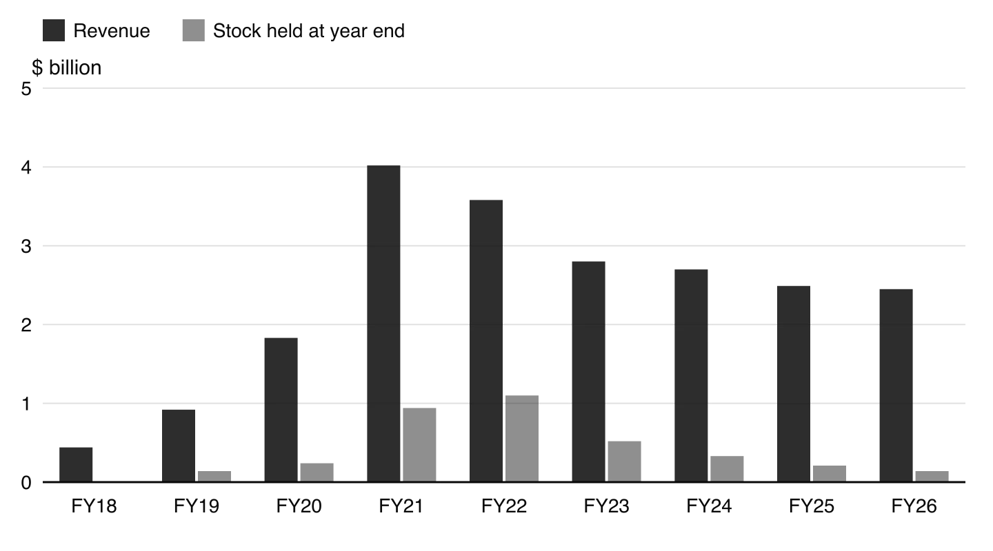
Peloton planned its capacity on the assumption that much of this growth would last. In May 2021 it announced Peloton Output Park, its first dedicated factory, in Troy Township, Ohio: a site of more than 200 acres with over one million square feet of space, expected to create more than 2,000 jobs and to start producing bikes and treadmills in 2023. In August 2021 it forecast revenue of $5.4 billion for FY2022.
As vaccines arrived and gyms reopened, demand fell well below that forecast. Peloton cut its FY2022 revenue forecast twice, and actual revenue was $3.58 billion, about 34% below the original forecast. Stock rose to $1.10 billion by June 2022, almost a third of the year’s revenue, and the company recorded $224.9 million of stock write-downs in FY2022.
Date of forecast | FY2022 revenue forecast ($bn) | Basis given by the company |
|---|---|---|
August 2021 | 5.4 | Growth to 3.63 million connected fitness subscriptions |
November 2021 | 4.4–4.8 | “A more pronounced tapering of demand” as the economy reopened |
February 2022 | 3.7–3.8 | Traffic trends from the first half of the year extended into the second |
Actual (year to June 2022) | 3.58 |
In February 2022 the company announced a restructuring: it would wind down the development of Peloton Output Park, reduce planned capital expenditure for 2022 by about $150 million and cut about 2,800 jobs, aiming for at least $800 million of annual cost savings. Its chief executive stepped down at the same time. Peloton made a net loss of $2.83 billion in FY2022; revenue kept falling, to $2.45 billion in FY2026, the year in which the company reported a net profit of $63.2 million after losses in every year from FY2018.
Our forecast extrapolates traffic trends from the first half of the year into the second and incorporates assumed demand impacts from reduced sales and marketing spend and the implementation of delivery and set-up surcharges on January 31st.
— Peloton Interactive, Inc., Q2 FY2022 shareholder letter, 8 February 2022
Time series analysis explains both the error and its cause. The pandemic surge was a random variation, a one-off shock, and not a change in the long-term trend. Extrapolating the growth of 2020–2021 treated it as a trend, and a factory designed for that demand would have added capacity just as demand fell. Moving averages would not have helped either: averages of the boom quarters would have shown a steep rising trend, because any method based only on past data assumes the conditions behind those data will continue.
The case also shows how forecasts drive the other functions. The over-forecast led to too much stock (operations), stock write-downs and losses (finance), job cuts (human resources) and price cuts (marketing). The limits of the evidence must be kept in mind: Peloton also faced a product recall in 2021 and stronger competition, so not all of the fall in revenue was a forecasting failure, and a business that had under-forecast would have lost sales to rivals during the boom. A sounder approach would have combined the data with qualitative judgment about how long gyms would stay closed, and planned capacity that could be scaled back.
Sources: Peloton Interactive, Inc., Form 8-K filings of 24 May 2021, 26 August 2021, 4 November 2021 and 8 February 2022 (press releases and shareholder letters); Form 10-K annual reports FY2019–FY2026, via SEC EDGAR, retrieved October 2026.
Explain why Peloton’s revenue growth in FY2021 was a poor guide to the trend in its sales.
Analyse how the overestimate of demand affected Peloton’s operations, finance and human resources.
To what extent could Peloton have avoided its forecasting error by using qualitative forecasting methods?
Exam practice
Sales forecasting questions appear only on HL papers, mainly Paper 2, usually with quarterly or monthly data in the stimulus. Typical questions ask you to define a term, calculate moving averages or seasonal variations, construct or complete a table or chart of the trend, use the result to forecast, and comment on or evaluate the reliability of the forecast for the business in the case.
The next question uses quarterly data from an invented business. Alpenrad is a small Swiss shop that sells and rents skis in winter and mountain bikes in summer. Its quarterly sales revenue (hypothetical data) is shown in the table.
Quarter | Q1 Y1 | Q2 Y1 | Q3 Y1 | Q4 Y1 | Q1 Y2 | Q2 Y2 | Q3 Y2 | Q4 Y2 |
|---|---|---|---|---|---|---|---|---|
Sales (CHF 000) | 80 | 30 | 40 | 90 | 88 | 34 | 46 | 96 |
Calculation questions are often followed by a short explanation question on the same business, which needs the data from the case.
Summary
A sales forecast predicts future sales in volume or value; production, stock, cash flow, budgets, workforce plans and finance all depend on it.
Qualitative methods (expert opinion, sales force composite, the Delphi method) rely on judgment; quantitative methods (time series analysis, extrapolation, simple linear regression) rely on past data.
A time series has four components: the trend, seasonal variation (within a year), cyclical variation (the business cycle) and random variation (one-off events).
Moving averages smooth out seasonal and random variation to show the trend; four-quarter averages must be centred.
Seasonal variation = actual − trend; a forecast = extrapolated trend + average seasonal variation for the period.
Forecasts help businesses plan, but they assume the past will continue, cannot predict shocks and become less reliable the further ahead they reach.
Forecasts are most useful for established products in stable markets over short horizons, especially when methods are combined and plans stay flexible.
Self-check
- To do:
I can define sales forecasting and explain how other functions of the business use a sales forecast.
- To do:
I can distinguish qualitative from quantitative forecasting and describe expert opinion, the sales force composite and the Delphi method.
- To do:
I can explain trend, seasonal, cyclical and random variation with an example of each.
- To do:
I can calculate three-period moving averages and centred four-quarter moving averages.
- To do:
I can calculate seasonal variations and average seasonal variations.
- To do:
I can forecast sales by extrapolating the trend and adding the average seasonal variation.
- To do:
I can explain how extrapolation and simple linear regression are used to forecast sales.
- To do:
I can evaluate the benefits and limitations of sales forecasting for a particular business.