4.12 Standardising normal variables · IB Maths AA | Augment Education
4.12 Standardising normal variables
Standardise normal variables with z = (x − μ)/σ, interpret z-values, compare values from different distributions, and find an unknown mean or standard deviation (or both) from given probabilities.
IB Mathematics: Analysis and Approaches
Part of 4 Statistics and probability
SL and HL
Key terms introduced here
Each is in the Maths AA glossary, with every other term in the subject.
The normal distribution with mean 0 and standard deviation 1, written Z∼N(0,1). Standardising any normal variable gives a variable with this distribution.
The number of standard deviations that a value x lies from the mean, z=σx−μ. A positive z-score means the value is above the mean; a negative one means it is below.
of a value
x
, and interpret it as a number of standard deviations from the mean.
Use z-values to compare values that come from different normal distributions.
State the properties of the standard normal distribution Z∼N(0,1), and explain why P(X<x)=P(Z<z).
Find probabilities and boundaries for any normal variable by standardising.
Determine an unknown mean or an unknown standard deviation from a given probability.
Solve simultaneous equations to find an unknown mean and standard deviation together.
Every normal distribution has the same shape. Two normal curves differ only in where they are centred and how widely they are spread, so measuring every value by its distance from the mean, in units of standard deviations, puts all of them on one common scale. This process is called standardising, and the result is a z-value.
Standardising has two main uses. It makes values from different distributions comparable, such as a score in one test and a score in another test marked in a different way. It also turns a question about an unknown mean or standard deviation into a linear equation, which is how a manufacturer sets a machine so that only a small fraction of its products are underweight.
The z-value
Measuring distance from the mean in standard deviations
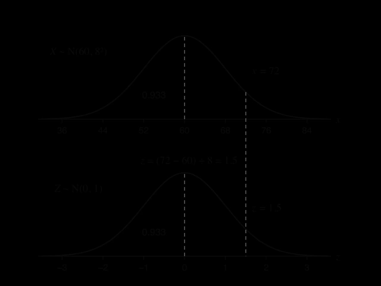
A score of 72 means little without its context. If the scores of a large group are modelled by X∼N(60,82), then 72 is 12 above the mean, and since each standard deviation is 8, it is 812=1.5 standard deviations above the mean. That number, 1.5, is the z-value of 72.
The formula is in the formula booklet. Its numerator is the distance from the mean, with a sign, and dividing by σ converts that distance into standard deviations. A z-value has no units: the units of x−μ and σ cancel.
z-value
Meaning
z=0
x equals the mean
z=1
x is one standard deviation above the mean
z=−2
x is two standard deviations below the mean
∣z∣>2
x is unusual: about 5% of values are this far from the mean
∣z∣>3
x is very rare: about 0.3% of values are this far from the mean
The last two rows come from the 68–95–99.7 rule (4.9). A z-value therefore gives a quick sense of how ordinary or extreme a value is, whatever the original units.
Going back from z to x
Rearranging the definition gives the value that has a particular z-value:
x=μ+zσ
In words, start at the mean and move z standard deviations: to the right if z is positive, to the left if it is negative. This form is the one used whenever z is known and x is wanted, including every inverse normal problem later in the subtopic.
Comparing values from different distributions
Two values measured on different scales cannot be compared directly, but their z-values can. The value with the larger z-value is further above its own mean, measured in its own standard deviations, so it is the better performance relative to its group.
The standard normal distribution
Standardising a normal variable
Standardising can be applied to the whole random variable as well as to single values. If X∼N(μ,σ2), define
Z=σX−μ
Subtracting μ moves every value left by μ, a translation, so the new mean is 0 and the shape and spread are unchanged. Dividing by σ then shrinks every distance from the mean by the factor σ, so the new standard deviation is 1. A translation and a scaling keep the shape of the bell, so Z is still normally distributed.
The graph of the standard normal distribution is centred on 0, has points of inflexion at z=±1, and in practice lies between z=−3 and z=3. Its z-values are measured in standard deviations, so the 68–95–99.7 rule reads directly off its axis.
Z ~ N(0, 1)
The standard normal curve is symmetric about z = 0. About 68% of its area lies between z = −1 and z = 1, and about 95% between the dashed lines at z = −2 and z = 2.
Why standardising keeps probabilities
The event X<x happens exactly when σX−μ<σx−μ, because subtracting μ and dividing by the positive number σ do not change the direction of an inequality. The two events are the same event, so they have the same probability:
P(X<x)=P(Z<σx−μ)=P(Z<z)
On a diagram, the shaded area under the curve of X to the left of x is equal to the shaded area under the standard normal curve to the left of z.
Standardising relabels the axis: 60 becomes 0, each step of 8 becomes a step of 1, and 72 becomes 1.5. The shaded areas are equal, so P(X < 72) = P(Z < 1.5).
With a GDC the two methods give identical answers, so standardising is not needed for probabilities with a known mean and standard deviation. It becomes necessary in two situations: when a probability for Z is given in the question instead of a GDC being available, and when μ or σ is unknown.
Inverse normal calculations with z
From a probability to z, then to x
The inverse normal function of a GDC works for any normal distribution, so a boundary can be found directly. It can also be found in two steps through Z: first find the z-value with the given area, using μ=0 and σ=1, then convert it with x=μ+zσ. The two-step method is the one that extends to an unknown μ or σ, so it is worth practising first where the answer can be checked.
Useful z-values
A few z-values occur so often that it helps to recognise them. Each is found from the inverse normal function of Z∼N(0,1), and the symmetry of the curve gives the negative values from the positive ones.
Area to the left of z
z
Typical use
0.9
1.2816
the top 10%
0.95
1.6449
the top 5%, or the middle 90%
0.975
1.9600
the middle 95%
0.99
2.3263
the top 1%
0.1, 0.05, 0.01
−1.2816, −1.6449, −2.3263
the bottom 10%, 5%, 1%
The middle 95% of any normal distribution lies within 1.96 standard deviations of the mean. The value 2 in the 68–95–99.7 rule is a rounded form of this.
Finding an unknown mean or standard deviation
The method
When μ or σ is unknown, the GDC's normal functions cannot be used directly, because they need both values. Standardising gets round this, because the inverse normal function of Z∼N(0,1) needs neither. The method has four steps.
Sketch the curve, mark the given boundary and shade the given probability.
Write the probability as an area to the left, and find the matching z-value from Z∼N(0,1).
Write the equation σx−μ=z, with the known values substituted.
Solve for the unknown, and check the answer with the normal cdf.
An unknown mean
If σ is known and μ is not, the equation σx−μ=z is linear in μ. A common application is setting a filling machine. The standard deviation depends on the machine's precision and is fixed, while the mean can be adjusted, and the question is how high to set it so that few packets fall below the stated mass.
In this setting, the extra 9.3 g in each packet is the cost of the machine's imprecision. A machine with a smaller standard deviation could be set to a lower mean with the same 1% guarantee, which is one reason manufacturers invest in more precise equipment.
An unknown standard deviation
If μ is known and σ is not, the equation is σx−μ=z with σ in the denominator. Multiply by σ and divide by z:
σ=zx−μ
Both x−μ and z have the same sign (both positive when x is above the mean, both negative when it is below), so σ comes out positive, as it must.
Using symmetry to find the mean
When two tails of equal probability are given, one on each side, symmetry gives the mean without any calculation: the mean is the midpoint of the two boundaries. Only the standard deviation then needs a z-value.
The same idea links a normal distribution to its quartiles and percentiles (4.2). The lower quartile has area 0.25 to its left and the upper quartile has area 0.75, so the quartiles are symmetric about the mean and lie 0.6745 standard deviations either side of it. The interquartile range of any normal distribution is therefore 2×0.6745σ≈1.35σ.
Finding both the mean and the standard deviation
Two conditions, two equations
When both μ and σ are unknown, one probability is not enough: it gives one equation in two unknowns. Two probabilities at two different boundaries give two equations, and because each equation σx−μ=z can be rewritten as
μ+zσ=x
they form a pair of linear simultaneous equations in μ and σ. These can be solved by elimination, by substitution or with the simultaneous equation solver of a GDC.
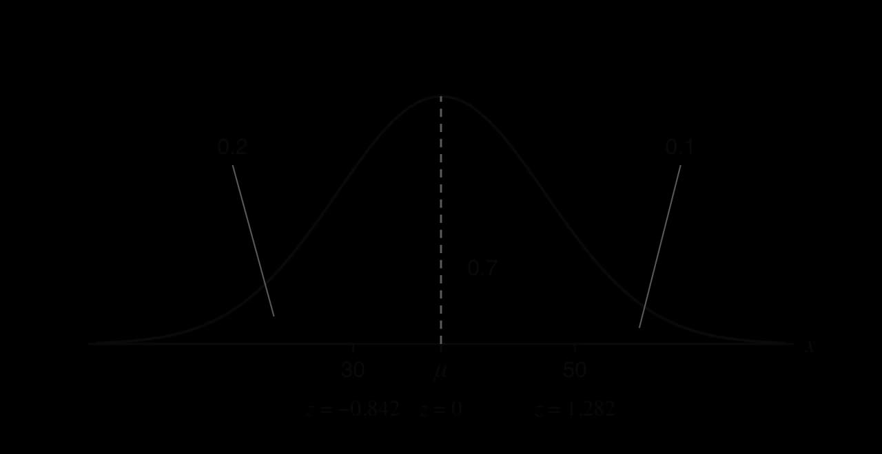
Each boundary is matched with its own z-value: 30 has area 0.2 to its left, so z = −0.842; 50 has area 0.9 to its left, so z = 1.282.
A quick check on the signs: in the figure, 30 is below the mean and 50 is above it, so the z-values must be negative and positive respectively, and the answer for μ must lie between 30 and 50. The value 37.9 does, and it is closer to 30 because the left tail (0.2) is larger than the right tail (0.1).
Two unknowns in context
In context, the two conditions are usually given as percentages of a population, often as classes such as "small" and "large". Each percentage becomes an area to the left, then a z-value, then an equation, exactly as in the abstract case.
Exam-style questions on standardising
Questions on standardising usually combine a context, a pair of given percentages and a follow-on part that uses the new parameters. The equations must be written out, because a GDC cannot find μ and σ in one step, and "show that" parts often ask for exactly those equations.
The second question gives the z-value in the question, as happens on papers where a GDC is not allowed. The method is the same; only the inverse normal step is replaced by the given value.
Self-check
To do:
I can calculate a z-value with z=σx−μ and interpret it as a number of standard deviations from the mean.
To do:
I can convert a z-value back to a value with x=μ+zσ.
To do:
I can use z-values to compare values from different normal distributions.
To do:
I can state that Z=σX−μ∼N(0,1) and explain why P(X<x)=P(Z<z)
To do:
I can find a z-value from a probability, choosing the correct sign.
To do:
I can find an unknown mean or an unknown standard deviation from one probability.
To do:
I can use symmetry to find the mean when two equal tails are given.
To do:
I can set up and solve simultaneous equations to find both μ and σ.
A1
(b)
Apples heavier than k grams are sold as “premium”. 15% of apples are premium. Find k.
[3]3 marks
Markscheme (b)
P(M>k)=0.15(M1)
z=1.0364(A1)
k=192 g (192.437…) A1
Question 2 · AA-0042015 marks
The lifetimes, T hours, of a brand of rechargeable battery are normally distributed with mean 40 hours and standard deviation σ hours. It is known that 10% of these batteries have a lifetime of less than 37 hours.
(a)
Show that σ=2.341, correct to four significant figures.
[3]3 marks
(b)
Find the probability that a randomly selected battery has a lifetime of more than 44 hours.
[2]2 marks
(c)
A battery has already lasted 42 hours. Find the probability that its lifetime is more than 45 hours.
[3]3 marks
(d)
Find the probability that at least 7 of the batteries in a randomly selected pack have a lifetime of at least 37 hours.
[3]3 marks
(e)
Given that at least one battery in a pack has a lifetime of less than 37 hours, find the probability that exactly two batteries in the pack have a lifetime of less than 37 hours.
The time taken for a ferry to cross a lake, T minutes, is normally distributed with mean 42 minutes and standard deviation σ minutes. It is found that 6% of crossings take longer than 47 minutes.
(a)
Find the value of σ.
[3]3 marks
(b)
Find the probability that a randomly chosen crossing takes less than 40 minutes.