Notes on 2.12 Polynomial functions
Polynomial functions are built from whole-number powers of only, so they are the simplest functions after straight lines and quadratics. Their graphs are smooth unbroken curves, they can be differentiated and integrated term by term, and many other functions are approximated by polynomials. Engineers use them to design smooth curves such as road transitions and roller-coaster profiles, and computers use them to draw fonts and animations.
What a polynomial is
A polynomial in is a sum of terms, each of which is a constant multiplied by a non-negative whole-number power of . Linear functions () and quadratic functions (
The degree is the highest power of that appears with a non-zero coefficient. A constant function such as is a polynomial of degree 0. The sum notation
An expression is not a polynomial if any power of is negative or a fraction, or if appears inside a root, a denominator, an exponent, a logarithm or a trigonometric function.
Expression | Polynomial? | Reason |
|---|---|---|
Yes | Degree 5, leading coefficient | |
Graphs of polynomial functions
Every polynomial is defined for all real , and its graph is a single smooth curve with no breaks, corners or asymptotes. The shape of the graph is controlled by three things: the degree, the sign of the leading coefficient, and the zeros with their multiplicities.
Turning points and zeros
A polynomial of degree has at most real zeros and at most turning points. A cubic can have two turning points or none (as has none), and a quartic can have three or one. The number of turning points of a polynomial of degree
A polynomial of odd degree always has at least one real zero, because its two ends go in opposite directions, so the unbroken graph must cross the -axis somewhere. A polynomial of even degree may have no real zeros at all, as shows.
End behaviour
For large positive or negative values of , the leading term is much larger in size than all the other terms put together. For example, when the polynomial
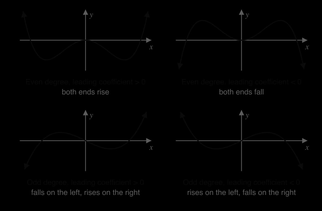
Degree |
|---|
The notation is read "as tends to infinity", meaning as becomes larger and larger without limit.
Zeros, roots and factors
The zeros of are the values of for which ; they are the roots of the equation and the
If for some polynomial , then
So the zeros can be read from a factorised form: has zeros ,
A polynomial of degree with real coefficients can always be written as a product of real linear factors and real quadratic factors that have no real roots. Each quadratic factor with a negative discriminant contributes two non-real roots, which are complex conjugates (see 1.14). Counting complex roots and repeats, a polynomial of degree has exactly roots.
Multiplicity
A factor may appear more than once. In the factor
Multiplicity decides how the graph meets the -axis. Near , the factor changes sign only if is odd, while the other factors keep roughly the same value. So the graph crosses the axis at a root of odd multiplicity and touches it, then turns back, at a root of even multiplicity.
Multiplicity of the root | Graph at |
|---|---|
1 (simple) | Crosses the -axis, looking like a straight line nearby |
2 (or any even number) | Touches the -axis and turns back: a turning point on the axis |
3 (or any odd number |
The higher the multiplicity, the flatter the graph is near the root. A root of multiplicity 2 or more is always a stationary point of the graph, since the gradient there is zero.
Sketching a polynomial from its factorised form
A sketch shows the general shape and the key features, labelled; it does not need to be accurate to scale. To sketch from a factorised form:
Find the -intercept by substituting .
Find the zeros and their multiplicities from the factors, and mark them on the -axis.
Find the end behaviour from the leading term.
Starting from the far left, draw a smooth curve that follows the end behaviour, crosses at odd-multiplicity roots, touches and turns at even-multiplicity roots, and finishes with the correct right-hand end behaviour. The curve must pass through the -intercept.
Between two neighbouring zeros the graph has at least one turning point. Its exact position needs calculus (5.8) or a graphic display calculator (GDC); a sketch only needs it in roughly the right place.
The same method works for higher degrees. With an even-degree polynomial both ends point the same way, so the number of crossings is even when every root is counted with its multiplicity.
Finding the equation from a graph
Reversing the process gives the equation from a graph. The zeros and their behaviour (crossing or touching) give the factors, and one more point on the curve, often the -intercept, gives the constant multiplier.
Polynomial division
To factorise a polynomial of degree 3 or more, or to simplify a rational function, one polynomial often has to be divided by another. Polynomial division works like the long division of numbers: gives quotient and remainder because
The symbol shows an identity: the two sides are equal for every value of . When the divisor is linear the remainder has degree 0, so it is a constant.
Long division
Long division repeats one cycle until the remainder has a lower degree than the divisor:
Divide the leading term of what is left by the leading term of the divisor. Write the result in the quotient.
Multiply the whole divisor by that term.
Subtract, and bring down the next term.
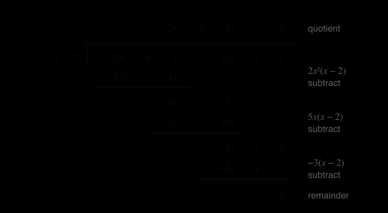
The division of by runs as follows.
. Multiply:
The remainder has degree 0, lower than the divisor, so the division stops:
The same cycle works for a quadratic divisor. The division stops when what is left has degree less than 2, so the remainder can be linear.
Synthetic division
Synthetic division is a short form of long division for a linear divisor . It keeps only the coefficients, because the powers of are fixed by their positions. To divide by :
Write on the left and the coefficients of in descending powers (with for any missing power).
Bring the first coefficient down.
Multiply it by , write the result under the next coefficient, and add.
Repeat step 3 to the end. The last number is the remainder; the others are the coefficients of the quotient, which has degree one less than
For , the divisor is
The bottom row gives the quotient and the remainder :
Synthetic division works because each step does exactly what long division does: bringing down and multiplying by is "divide the leading term by , then multiply by ", and adding instead of subtracting accounts for the sign of .
Comparing coefficients
A division can also be done by writing the identity with unknown coefficients and comparing the coefficients of each power of . For
Expanding the right side gives
The remainder theorem
When the divisor is linear, the remainder can be found without dividing at all. Put in the division identity. The remainder is a constant , so
This holds for every , so it holds for , where the first term vanishes:
The second form follows in the same way: is zero when . The remainder theorem turns a long division into a single substitution.
Finding unknown coefficients from remainders
Each piece of information about a remainder gives one equation. One unknown needs one condition; two unknowns need two conditions, which then form a pair of simultaneous equations.
The polynomial leaves remainder
Adding the two equations gives , so and .
The factor theorem
A remainder of zero means the divisor is a factor. Applying this to the remainder theorem gives the factor theorem, the main tool for factorising polynomials of degree 3 or more.
"If and only if" means the statement works in both directions: a factor gives a zero, and a zero gives a factor.
Factorising a cubic
To factorise a cubic with integer coefficients, search for one zero, use it to find a linear factor, divide, and then factorise the quadratic quotient.
If a polynomial with integer coefficients has a rational root in lowest terms, then divides the constant term and divides the leading coefficient. So the candidates to try are the fractions
In a "show that" question, the conclusion must be stated in words, and every step of the substitution must be visible. A line such as "" on its own does not show the working.
Finding unknown coefficients from factors
If and are both factors, then so is their product, and each gives one equation. A quadratic factor
Remainders on division by a quadratic
When the divisor is a quadratic, the remainder is linear, , so two conditions are needed. If the quadratic factorises as , substituting
Sum and product of the roots
The coefficients of a polynomial carry information about its roots even when the roots themselves are hard to find. The link comes from expanding the factorised form.
Deriving the results
A quadratic with roots and can be written
Comparing coefficients, and , so
A cubic with roots ,
Comparing coefficients gives
The same expansion for degree produces the coefficient for and
The product formula changes sign with the degree. For a quadratic or a quartic ( even) the product is ; for a cubic or a quintic (
Using the sum and product to find roots and coefficients
The formulas are most useful when some extra information links the roots: one root is known, the roots form a sequence, or two roots are related.
When the coefficients are real, non-real roots come in conjugate pairs (the conjugate root theorem, 1.14). Combined with the sum and product, one complex root is often enough to find all the others.
Polynomial models
Polynomials model quantities that are built from products of lengths, such as volumes, and smooth curves that are fitted through measured points. In a model, the mathematical solutions must be checked against the context: a length cannot be negative, and a model is valid only over a sensible domain.
The domain matters here: the height must be positive, so the model only makes sense for . A polynomial that fits data well over a measured range can give absurd values outside it, because its end behaviour sends it to ; extrapolating far beyond the data is unreliable.
Exam-style questions on polynomial functions
The following question is typical of Paper 1 (no GDC), where the factor theorem, division and sketching are tested together.
On Paper 2 a GDC is available. Its polynomial solver finds all the roots of a polynomial equation, including complex ones on most models, and its graphing tools find intercepts and turning points. A question that says "find" on Paper 2 can be answered with the GDC, but a sketch copied from the screen still needs its intercepts and turning points labelled, and answers must be given exactly or to 3 significant figures.
Self-check
- To do:
I can state the degree, leading coefficient and constant term of a polynomial, and recognise expressions that are not polynomials.
- To do:
I can describe the end behaviour of a polynomial from its degree and the sign of its leading coefficient.
- To do:
I can sketch a polynomial from its factorised form, showing where it crosses or touches the -axis.
- To do:
I can find the equation of a polynomial from its graph, including the constant multiplier.
- To do:
I can divide a polynomial by a linear or quadratic divisor using long division or synthetic division.
- To do:
I can use the remainder theorem to find a remainder, and both theorems to find unknown coefficients.
- To do:
I can factorise a cubic or quartic by finding a root with the factor theorem and dividing.
- To do:
I can find the sum and the product of the roots of a polynomial equation and use them to find unknown roots or coefficients.