2.10 Solving equations

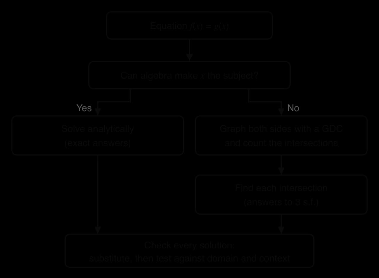
Solving an equation means finding every value of the unknown that makes it true. Some equations, such as $2x + 5 = 11$ or $x^2 - 5x + 6 = 0$, can be solved exactly with algebra. Many others, including some that look simple, such as $e^x = 3 - x^2$ or $\sin x = \frac{x}{2}$, cannot be rearranged to make $x$ the subject at all; they can only be solved approximately, by graphs or by technology.

A reliable approach to any equation uses both views. Algebra gives exact answers where it can, and the graph shows how many solutions there are and roughly where they lie, so that none is missed. In applications, the solutions then need to be interpreted: a model may produce values that make no sense in the real situation, and these must be rejected.

Analytic and graphical solutions

What a solution is

A solution (or root) of an equation is a value of the unknown that makes the two sides equal. The set of all solutions is the solution set, and it may contain no values, one value, several values or infinitely many. For example, $x^2 = 4$ has the solution set $\{-2, 2\}$, while $x^2 = -4$ has no real solutions.

There are two kinds of answer, depending on the method.

An analytic solution is exact and shows the structure of the answer, so it is preferred whenever algebra can produce one. A numerical solution is the only option when no algebraic method can isolate the unknown, and it is often the quicker route when a graphic display calculator (GDC) is available and an exact value is not asked for. In practice the two are used together: the analytic answer $x = \ln 3$ can be checked by evaluating it as $1.0986\ldots$ and comparing with a graph.

The graphical meaning of a solution

Any equation in one unknown can be written as $f(x) = g(x)$, with an expression on each side. Each side defines a graph, $y = f(x)$ and $y = g(x)$, and at a point where the graphs meet, both have the same $y$-value for the same $x$-value. So:

• the solutions of $f(x) = g(x)$ are the $x$-coordinates of the points of intersection of $y = f(x)$ and $y = g(x)$;

• the number of solutions equals the number of intersection points.

Moving everything to one side gives a second graphical view. The equation $f(x) = g(x)$ is equivalent to $f(x) - g(x) = 0$, so its solutions are the zeros of the function $h(x) = f(x) - g(x)$, the $x$-intercepts of $y = h(x)$. Both views give the same solutions, as the graphs of the equation $x^2 = x + 2$ show.

The algebra agrees: $x^2 - x - 2 = (x - 2)(x + 1) = 0$ gives $x = -1$ or $x = 2$. The solutions are the $x$-coordinates only. The intersection points $(-1, 1)$ and $(2, 4)$ are not themselves solutions of the equation.

Solving from a given graph

When a graph is printed with a question, solutions can be read from it to the accuracy that the scale allows. The method is to draw (or imagine) the graph of the other side of the equation and read the $x$-coordinates of the intersections. An equation such as $f(x) = 3$ is solved by drawing the horizontal line $y = 3$; an equation such as $f(x) = x$ by drawing the line $y = x$.

The graph of $y = x^3 - 3x$ for $-2.5 \le x \le 2.5$ has a local maximum at $(-1, 2)$ and a local minimum at $(1, -2)$. It is used in the next example.

The method in part (c) works for any equation of the form $f(x) = k$: slide a horizontal line up and down the graph and count the intersections. The changes in the number of solutions happen at the turning points and at any asymptotes.

Choosing a method

The first step with any equation is to decide whether algebra can solve it. The table lists the common types and their methods.

An equation has an analytic solution when the unknown can be isolated, which usually means it appears in only one "kind" of place. In $e^x = 3 - x^2$ the unknown is both in an exponent and in a polynomial; taking logarithms gives $x = \ln(3 - x^2)$, which still has $x$ on both sides, and no algebraic step removes it. Such equations are solved numerically.

Solving equations analytically

Exact solutions by algebra

Analytic methods transform an equation into simpler equivalent equations until the unknown is isolated. Each step must be reversible, or every answer checked at the end, because some steps can create or lose solutions.

When the unknown appears in the same expression more than once, a substitution may turn the equation into a familiar type. An equation in $e^{2x}$ and $e^x$ is a quadratic in $e^x$, because $e^{2x} = \left(e^x\right)^2$.

Solutions that must be rejected

Some algebraic steps produce values that do not satisfy the original equation. Combining logarithms is one example: $\ln x + \ln(x - 2)$ is only defined when $x > 0$ and $x > 2$, but the combined form $\ln\big(x(x - 2)\big)$ is also defined when $x < 0$. Squaring both sides of an equation is another: $x = 3$ has one solution, but $x^2 = 9$ has two.

Solving equations with technology

Equations with no analytic method

Consider the equation $e^x = 3 - x^2$. The graphs of $y = e^x$ and $y = 3 - x^2$ show at once that there are exactly two solutions, one negative and one positive. The exponential curve is always positive and increasing, while the parabola has a maximum of 3 at $x = 0$, so they cross once on each side of the $y$-axis and never again: for $x > 0.9$ the parabola is already below the exponential and falling, and for $x < -1.8$ it is negative.

A GDC finds each intersection to many decimal places: $x = -1.677\,23\ldots$ and $x = 0.834\,487\ldots$, so to 3 significant figures $x = -1.68$ or $x = 0.834$. No algebraic method can give these values exactly.

Three ways to solve with a GDC

A GDC offers three methods. All give the same values; they differ in how much they show and how easily a solution can be missed.

For $e^x = 3 - x^2$, the zero method uses $h(x) = e^x + x^2 - 3$, whose $x$-intercepts are at the same two values. The numerical solver started from a guess of 1 returns only $0.834\ldots$; the negative solution appears only if a second guess, such as $-2$, is tried. For this reason, always graph first: the graph shows how many solutions to look for, and then each one can be found with whichever method is convenient.

Equations involving trigonometric functions

The same methods apply to equations containing trigonometric functions. Calculations use radians unless the question uses degrees (see 3.4 and 3.8), and the GDC must be set to the matching mode.

Deciding the number of solutions without solving

Sometimes the number of solutions can be found by reasoning about the graphs, without any calculation. Two useful facts are:

• an increasing function and a decreasing function meet at most once;

• if $f(x) - g(x)$ changes sign between $x = a$ and $x = b$, and both functions are continuous there, the graphs cross at least once between $a$ and $b$.

For example, $\ln x = 2 - x$ has exactly one solution: $\ln x$ is increasing, $2 - x$ is decreasing, and at $x = 1$ the left side is smaller ($0 < 1$) while at $x = 2$ it is larger ($0.693 > 0$). The GDC gives the solution $x \approx 1.56$.

Equations in context

Solving, interpreting and checking

When an equation comes from a model, solving it is only part of the work. The process has four stages:

1. Form the equation from the model and the condition in the question ("when does the population reach 50 000?" becomes $P(t) = 50$ if $P$ is in thousands).

2. Solve it, analytically or with technology.

3. Interpret each solution in the context: what it means, in the right units, and to a sensible accuracy.

4. Reject solutions that are impossible: negative times or lengths, values outside the domain of the model, or values beyond the range where the model is valid.

The domain of a model is often set by the context rather than by the algebra, so every solution should be compared with it. A model of a ball's flight is valid only while the ball is in the air; a model of a business is valid only for whole numbers of items sold, and only up to the capacity of the factory.

Break-even and intersection models

A common application compares two quantities modelled by different functions: cost and revenue, supply and demand, or two competing populations. The values at which they are equal are the solutions of an equation, and the graphs show which quantity is larger on each side of these values.

The next model cannot be solved with algebra, because time appears both in an exponent and in a linear term.

This comparison of linear and exponential growth is a pattern that appears in many models: whatever the starting values, an exponentially growing quantity eventually overtakes any linearly growing one.

Rejecting impossible solutions

Geometry and measurement models often produce solutions that are mathematically correct but physically impossible. A length or a time must be positive, and the dimensions of an object must all be positive at once.

Equations with two meaningful solutions

When a quantity rises and then falls, it passes through most values twice, and both solutions can be meaningful. Together they usually describe an interval of time during which some condition holds.

Exam-style questions on solving equations

The first question can be answered without a GDC and uses a "hence" link between parts; the second is a typical GDC question on intersections.

Self-check

• To do:

  I can explain why the solutions of $f(x) = g(x)$ are the $x$-coordinates of the intersections of $y = f(x)$ and $y = g(x)$.

• To do:

  I can decide whether an equation can be solved analytically, and choose a suitable method.

• To do:

  I can solve equations that reduce to quadratics, including those in $e^x$ or $2^x$, and give exact answers.

• To do:

  I can recognise and reject solutions that fall outside the domain of the original equation.

• To do:

  I can solve an equation with a GDC by the intersection method or the zero method, and find every solution.

• To do:

  I can find the number of solutions of $f(x) = k$ from a graph, including the values of a parameter $k$ that give a certain number of solutions.

• To do:

  I can form an equation from a model, solve it, interpret the solutions in context and reject impossible ones.

[3]3 marks

(b) Factorise: $x(x^2 - 3) = 0$, so $x = 0$ or $x^2 = 3$. The solutions are $x = -\sqrt{3}$, $0$ and $\sqrt{3}$.

(c) The solutions of $x^3 - 3x = k$ are where the horizontal line $y = k$ meets the curve. The line meets the curve three times when it lies strictly between the local minimum and local maximum values. At $k = 2$ or $k = -2$ the line touches a turning point and there are only two solutions; for $k > 2$ or $k < -2$ there is one. So there are exactly three solutions when $-2 < k < 2$.

• y = 2ˣ
• y = x²

• y = sin x
• y = x/2

Multiply by 20 to clear the decimals: $x^2 - 500x + 40\,000 = 0$, which factorises as $(x - 100)(x - 400) = 0$. So $x = 100$ or $x = 400$; both lie in the domain. The company breaks even when it makes 100 items or 400 items.

(b) The company makes a profit where $R(x) > C(x)$, that is where the revenue curve lies over the cost line. Between the break-even points, at $x = 200$ for example, $R = 6000$ and $C = 5000$, so the profit region is $100 < x < 400$: from 101 to 399 items.

(c) The study starts at $t = 0$, so the domain of the model is $t \ge 0$. A negative value of $t$ refers to a time before the study began, where the model was not intended to apply, so it is rejected.

(b) $V = 3(10 - 6)^2 = 3 \times 16 = 48$ cm³.

(c) Solve $x(10 - 2x)^2 = 48$. Expanding gives $x(100 - 40x + 4x^2) = 48$, so

Part (b) shows that $x = 3$ is a solution, so $x - 3$ is a factor. Dividing, $x^3 - 10x^2 + 25x - 12 = (x - 3)(x^2 - 7x + 4)$, and the quadratic formula gives

so $x \approx 0.628$ or $x \approx 6.37$. (A GDC gives the same three solutions of the cubic directly.) The value $6.37$ is rejected because it is not less than 5: the base would have side $10 - 2(6.37) < 0$. The volume is 48 cm³ when $x = 3$ or $x = \frac{7 - \sqrt{33}}{2} \approx 0.628$.

• V(t) = 600te^(−0.4t)

(b) Factorise: $(u - 2)(u - 4) = 0$, so $u = 2$ or $u = 4$. Then $2^x = 2$ gives $x = 1$, and $2^x = 4$ gives $x = 2$.

(c) The equation $4^x + 8 = 6 \times 2^x$ is the equation in part (a) rearranged, so the graphs meet where $x = 1$ and $x = 2$. Substituting into $y = 6 \times 2^x$: when $x = 1$, $y = 12$; when $x = 2$, $y = 24$. The points are $(1, 12)$ and $(2, 24)$. Check in the other equation: $4 + 8 = 12$ and $16 + 8 = 24$.

(b) The graphs meet twice, so there are 2 solutions.

(c) Using the intersect function of the GDC: $x = -0.398\,59\ldots$ and $x = 2.652\,93\ldots$, so $x = -0.399$ or $x = 2.65$ (3 s.f.).

(d) $f(x) > g(x)$ where the graph of $f$ is higher than the graph of $g$, which is between the intersections: $-0.399 < x < 2.65$.

$\sin\alpha = \frac{4}{\sqrt{160}}$ A1

$\sin\alpha = \frac{1}{\sqrt{10}}$ AG

Find the value of $x$ for which $\mathrm{C\hat{A}B} = 90°$.

[2]2 marks