Notes on B4.1 Fundamentals of ADTs
Learning objectives
Explain the properties and purpose of abstract data types (ADTs), and how one ADT can have several implementations. (HL only)
Sketch singly, doubly and circular linked lists, showing insertion, deletion, traversal and search step by step. (HL only)
Construct programs that insert, delete, traverse and search singly, doubly and circular linked lists. (HL only)
Evaluate linked lists against arrays and other structures in terms of memory use and performance. (HL only)
Explain how a binary search tree (BST) organises data, and sketch the tree produced by a sequence of insertions and deletions. (HL only)
State the in-order, pre-order and post-order traversals of a binary tree, and explain what each is used for. (HL only)
Construct programs that use sets: membership, add, remove, union, intersection, difference, subset and superset, with and without built-in set types. (HL only)
Explain how hash tables work: hash functions, collisions, separate chaining, linear probing, load factors and rehashing. (HL only)
Trace the insertion of keys into a hash table, and use
HashMapandHashSetin Java ordictandsetin Python. (HL only)Evaluate which ADT suits a given problem, using the Big O cost of its operations. (HL only)
Introduction
Programs that handle large or changing collections of data need more than arrays and lists. A music app moves backwards and forwards through a playlist, a spell checker tests whether a word exists among hundreds of thousands, and a social network works out which friends two users have in common. Each task is fast and simple with the right structure, and slow or awkward with the wrong one.
An abstract data type describes a collection by the operations it offers, separately from how it is stored, so a programmer can choose the operations a problem needs first and the storage that makes them fast second. Linked lists, binary search trees, sets and hash tables are the building blocks behind the standard libraries of most modern languages, including Java's LinkedList, HashMap and HashSet and Python's dict and set. They extend the arrays, stacks and queues of subtopic B2.2, Data structures, and use the Big O notation and recursion of subtopic B2.4, Programming algorithms.
Abstract data types
What an ADT specifies
Every collection a program uses has two sides. Its interface (in the general sense, not only Java's interface keyword) is what the rest of the program sees: the values the collection holds and the operations it can carry out. Its implementation is what happens inside: the arrays, references and variables that store the values, and the code of each operation. An abstract data type is the interface on its own, written down before any implementation is chosen.
The stack from subtopic B2.2 is the standard first example. As an ADT it is fully described by four operations and their effect, with no mention of arrays, indices or memory. The specification table lists each operation with what it takes, what it returns and what must be true before it is called (its precondition).
Operation | Input | Output | Effect | Precondition |
|---|---|---|---|---|
| an item | none |
| the stack is not full (bounded stacks only) |
| none | the top item | the top item is removed | the stack is not empty |
| none | the top item | none | the stack is not empty |
| none |
| none | none |
A program that uses only these four operations cannot tell how the stack is stored. Every other ADT is specified in the same way, from the queue of subtopic B2.2 to sets and maps; the table of common ADTs gives the core operations of each and the structures most often used to implement them.
ADT | Core operations | Typical implementations |
|---|---|---|
Stack | push, pop, peek, isEmpty | array with a top index; linked list (top = head) |
Queue | enqueue, dequeue, front, isEmpty | circular array; linked list with head and tail |
List | get(i), insert(i, x), remove(i), size | dynamic array ( |
Set | add, remove, contains, union, intersection, difference | hash table ( |
Map (dictionary) | put(key, value), get(key), remove(key), containsKey | hash table ( |
Tree | insert, delete, search, traverse | linked nodes with child references |
One ADT, several implementations
The stack diagram shows a program on top, the stack ADT's four operations in the middle, and two different implementations underneath. The program only ever calls the operations, so either implementation can be plugged in without changing a line of the program.
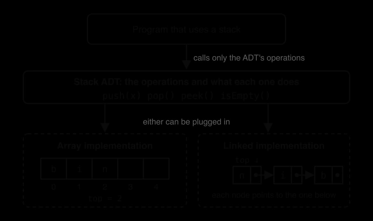
The program reverse_word uses a stack to reverse a word. It is written once, against the stack's operations, and then called with two completely different stack classes. ArrayStack stores the items in a fixed-size list with a top index; LinkedStack stores each item in a node holding a reference to the node beneath it, the building block of a linked list.
Python
class ArrayStack:
    """Stack ADT stored in a fixed-size list with a top index."""

    def __init__(self, capacity):
        self.items = [None] * capacity
        self.top = -1

    def is_empty(self):
        return self.top == -1

    def push(self, item):
        if .top == (.items) - :
             OverflowError()
        .top = .top +
        .items[.top] = item

     ():
         .is_empty():
             IndexError()
        item = .items[.top]
        .top = .top -
         item

     ():
         .is_empty():
             IndexError()
         .items[.top]


 :
     ():
        .data = data
        . =


 :


     ():
        .top =

     ():
         .top

     ():
        node = StackNode(item)
        node. = .top
        .top = node

     ():
         .is_empty():
             IndexError()
        item = .top.data
        .top = .top.
         item

     ():
         .is_empty():
             IndexError()
         .top.data


 ():

     letter  word:
        stack.push(letter)
    result =
      stack.is_empty():
        result = result + stack.pop()
     result


(reverse_word(ArrayStack(), ))
(reverse_word(LinkedStack(), ))
Java version
Java
interface StringStack {
    boolean isEmpty();
    void push(String item);
    String pop();
    String peek;
}

    {
     String[] items;
        -;

      {
        items =  [capacity];
    }

       {
         top == -;
    }

       {
         (top == items.length - ) {
              ();
        }
        top = top + ;
        items[top] = item;
    }

     String  {
         (isEmpty()) {
              ();
        }
           items[top];
        top = top - ;
         item;
    }

     String  {
         (isEmpty()) {
              ();
        }
         items[top];
    }
}

  {
    String data;
    StackNode next;

    StackNode(String data) {
        .data = data;
    }
}

    {
        ;

       {
         top == ;
    }

       {
            (item);
        node.next = top;
        top = node;
    }

     String  {
         (isEmpty()) {
              ();
        }
           top.data;
        top = top.next;
         item;
    }

     String  {
         (isEmpty()) {
              ();
        }
         top.data;
    }
}

   {

     String  {
         (   ; i < word.length(); i++) {
            stack.push(word.substring(i, i + ));
        }
           ;
         (!stack.isEmpty()) {
            result = result + stack.pop();
        }
         result;
    }

        {
        System.out.println(reverseWord( (), ));
        System.out.println(reverseWord( (), ));
    }
}
Both calls print the same result, because push, pop and isEmpty behave identically in the two classes.
Plain text
yranib
yranib
The two languages express the ADT differently. Java writes it down as an interface, StringStack, which lists the method signatures with no bodies; each class declares implements StringStack, and the compiler refuses to compile a class that leaves out an operation. The parameter of reverseWord has the interface as its type, so any class that implements it can be passed in. Python has no compulsory interface: any object with push, pop and is_empty methods works, and a missing method is found only when it is called. An abstract class from Python's abc module can enforce the same contract when that check matters.
Java's own collections library is built in exactly this way. List is an interface, and ArrayList (a dynamic array) and LinkedList (a doubly linked list) are two implementations of it. A program declares List<String> names = new ArrayList<>();; changing ArrayList to LinkedList in that one place swaps the implementation, and every other line still compiles, because every other line uses only List operations. The angle brackets give the type of item the list holds.
Why ADTs are used
Separating the interface from the implementation brings several practical benefits.
Abstraction. Programmers reason about a stack as push and pop, not as index arithmetic, so programs are shorter and easier to check.
Encapsulation. The stored data is reached only through the operations, so other code cannot corrupt it, for example by changing the top index of a stack without moving an item.
Interchangeable implementations. The implementation can be replaced, to save memory or to make a slow operation faster, without changing the code that uses it, as the switch between
ArrayListandLinkedListshows.Modularity and teamwork. One programmer can write code that uses a map while another writes the map, as long as both agree on the interface first.
Reuse. A well-tested ADT, such as Java's
HashMap, is written once and reused in millions of programs.Reasoning about correctness and cost. Each operation has a stated effect and a known Big O cost, so a designer can predict how a program behaves before running it.
The separation has limits. An interface states what an operation does but not how long it takes, and two implementations of the same ADT can differ greatly in speed. Removing the first item of a Python list with pop(0) and removing the first item of a linked list give the same result, but the first shifts every remaining element () while the second changes one reference (). A designer who ignores the implementation entirely can choose a structure that is correct but far too slow, so the cost of each operation is treated as part of the choice of ADT.
Linked lists
Nodes and pointers
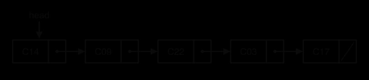
An array keeps its elements side by side in one block of memory, so any element's address can be calculated from its index. A linked list instead stores each item in its own small object, called a node, wherever free memory is found, and each node records where the next node is.
The memory diagram is a simplified model (real addresses, element sizes and object layouts differ by language and machine) showing the same four values stored both ways. In the array, the address of any element follows from its index. In the linked list, the nodes sit at unrelated addresses (3040, 1200, 5520, 2312), and each node's second field holds the address of the next one. The last node holds a special value, null in Java and None in Python, which marks the end of the list.

Neither Java nor Python exposes raw memory addresses. A node's reference field holds an object reference, which plays exactly the role of an address: it says where the next node is without the programmer ever seeing the number. In textbooks and diagrams this reference is called a pointer and is drawn as an arrow.
A linked list is reached through one or two pointers kept outside the nodes; without a pointer to the first node, the program could reach none of them.
Many implementations also keep a pointer to the last node, so that adding at the end does not require walking the whole list.
Singly linked lists
The simplest linked list gives each node one pointer, to the next node, so the list can only be followed in one direction, from head to tail.

The class Node holds one item and the reference to the next node. The class SinglyLinkedList holds the head and tail pointers and a count of nodes, and provides the four basic operations: traversal, search, insertion and deletion. Both versions are complete programs.
Python
Java version
Java
Running either version gives the same output (Java prints null and lower-case true/false where Python prints None, True and False).
Plain text
12 -> 25 -> 31 -> 47 -> None
5 -> 12 -> 25 -> 31 -> 47 -> 60 -> None
31 is at position 3
Delete 5: True
Delete 31: True
Delete 99: False
12 -> 25 -> 47 -> 60 -> None
size 4 tail 60
Traversal
Every operation except insertion at the head or tail starts with a traversal: a temporary reference, current, starts at the head and moves one node at a time with current = current.next until it becomes null/None. The loop condition tests current, not current.next, so the last node is processed before the loop ends.
Search
Search is a linear search along the chain: each node's data is compared with the target, stopping at the first match. It returns the position (or a Boolean, or the node itself) if found and a "not found" value such as −1 if the traversal reaches the end. Its cost is in the worst case, even when the list is sorted. Binary search needs to jump straight to the middle element, and a linked list can reach the middle only by walking half of it, so sorting a linked list does not make search .
Insertion at the head
Adding a node at the front takes two pointer changes, and their order matters. The new node must first be pointed at the current first node; only then is the head moved to the new node. The insertion diagram shows the list before, after step 1 and after step 2.
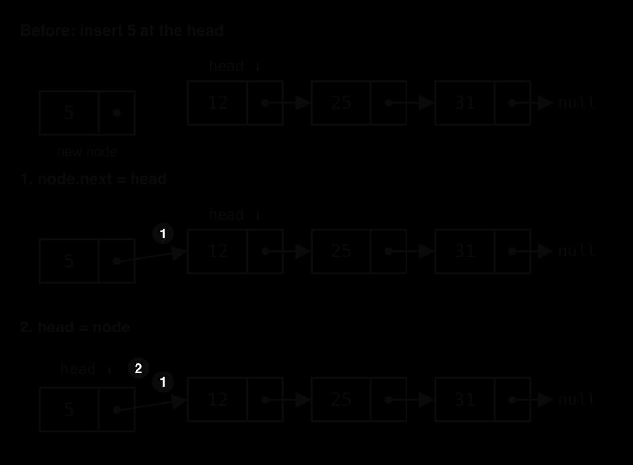
If the steps were swapped, head = node would run first and overwrite the only reference to node 12, leaving node 12 and everything after it unreachable (Java and Python then reclaim their memory automatically). When the list is empty, head is None, so step 1 sets the new node's next to None, which is exactly right for a one-node list; the code also sets tail, because the new node is now both first and last.
Insertion at the tail
With a tail pointer, appending is also : the old last node's next is set to the new node, then tail moves to the new node. Without a tail pointer, the program must first traverse the whole list to find the last node, which makes appending . An empty list is again a special case, because there is no old last node whose next can be set; the new node becomes both head and tail.
Insertion after a given node
Inserting in the middle, for example to keep a list in ascending order, has two stages. A traversal first finds the node after which the new value belongs, called current; this costs . The insertion itself is then two pointer changes, , in the same safe order as at the head: the new node is pointed at its successor first, and the predecessor is pointed at the new node second.
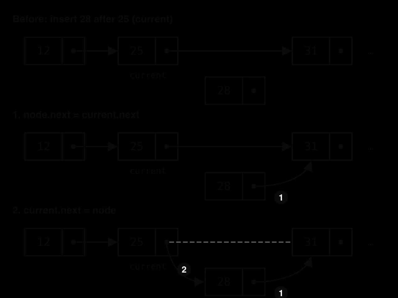
insert_sorted stops its traversal one node early: it tests current.next.data < value so that current ends at the predecessor, the only node whose pointer must change. A singly linked list has no way to step backwards, so a traversal that stopped on the successor would be one node too far.
Deletion
Deleting a node means making the chain skip it: the node before it, previous, takes over the deleted node's next reference with one assignment, previous.next = current.next. Nothing points to the deleted node any longer, so it disappears from every traversal. The deletion diagram shows this bypass, and the separate case of deleting the first node, where the head pointer moves on instead.
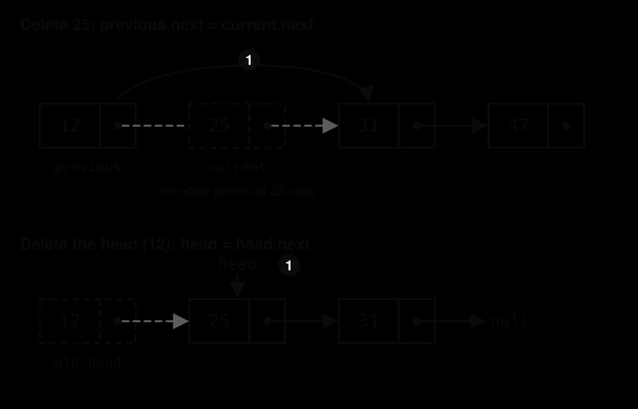
A complete deletion method handles four cases, each visible in the code of delete:
Empty list.
headisNone; there is nothing to delete, so returnFalsestraight away (otherwiseself.head.datawould raise an error).Target is the head. Move
headtohead.next. If the list is now empty, settailtoNoneas well.Target is later in the list. Walk two references,
previousandcurrent, one node apart; whencurrentholds the target, setprevious.next = current.next. Ifcurrentwas the tail,previousbecomes the new tail.Target not present. The loop reaches the end without a match; return
Falseand change nothing.
Doubly linked lists
A singly linked list cannot go backwards: to delete a node, the program needs its predecessor, and the only way to find the predecessor is to walk from the head. A doubly linked list removes that limitation by giving every node a second pointer, to the node before it.
Each node now has three fields: prev, the data and next. Every link between two neighbours appears twice, once in each direction, and both copies must be kept consistent: if node A's next is B, then B's prev must be A. Insertion therefore changes four pointers instead of two, as the insertion diagram shows for a playlist in which "Tide" is added after "Rain".
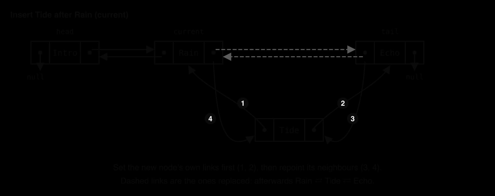
The order follows the same rule as before: the new node's own links are set while the old links still exist, and the old links are overwritten last. Step 3 uses current.next.prev, which is only correct while current.next still refers to Echo, so step 4 (current.next = node) must come after it. When the new node goes after the tail, there is no successor to update in step 3; instead, tail moves to the new node.
Deletion becomes simpler than in a singly linked list. A doubly linked node holds references to both of its neighbours, so a program that already holds a reference to the node can unlink it in without searching for the predecessor. Two assignments make the neighbours skip it.
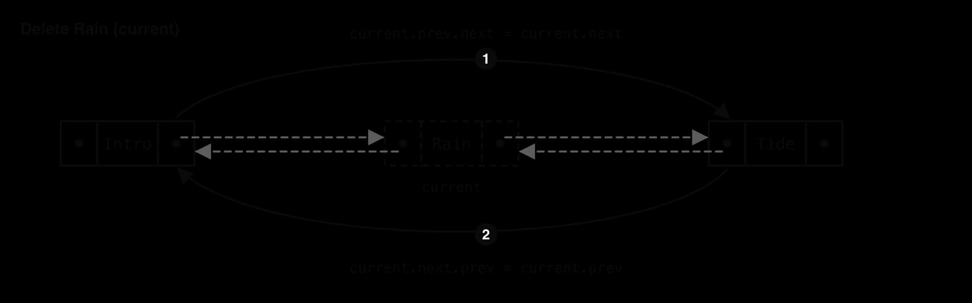
The class DoublyLinkedList stores a playlist of song titles. insert_after and delete follow the two diagrams, including the cases where the node is at either end, and display_backward starts at the tail and follows prev pointers, which is impossible in a singly linked list.
Python
class DNode:
    def __init__(self, data):
        self.data = data
        self.prev = None
        . =


 :
     ():
        .head =
        .tail =

     ():
        node = DNode(value)
         .head  :
            .head = node
            .tail = node
        :
            node.prev = .tail
            .tail. = node
            .tail = node

     ():
        current = .head
         current     current.data != target:
            current = current.
         current

     ():
        current = .find(target)
         current  :

        node = DNode(value)
        node.prev = current
        node. = current.
         current.   :
            current..prev = node
        :
            .tail = node
        current. = node


     ():
        current = .find(target)
         current  :

         current.prev   :
            current.prev. = current.
        :
            .head = current.
         current.   :
            current..prev = current.prev
        :
            .tail = current.prev


     ():
        current = .head
        text =
         current   :
            text = text + current.data +
            current = current.
        (, text)

     ():
        current = .tail
        text =
         current   :
            text = text + current.data +
            current = current.prev
        (, text)


playlist = DoublyLinkedList()
 song  [, , ]:
    playlist.append(song)
playlist.insert_after(, )
playlist.display_forward()
playlist.delete()
playlist.delete()
playlist.display_forward()
playlist.display_backward()
Java version
Java
Java compares the strings with equals, because == on two String objects compares references, not contents. The output shows the list read in both directions after deleting the head ("Intro") and the tail ("Echo"):
Plain text
Forward:  Intro Rain Tide Echo
Forward:  Rain Tide
Backward: Tide RainJava's own LinkedList class is documented as a "doubly-linked list implementation of the List and Deque interfaces", so the same structure serves as a list, a stack and a queue. Python's built-in list is not linked at all: the Python documentation describes CPython lists as "variable-length arrays, not Lisp-style linked lists", which is why a Python list's pop(0) is while removing the first node of a linked list is .
Circular linked lists
In a circular linked list, the last node's pointer leads back to the first node instead of to null. The list then has no end: a traversal can go round and round, which is exactly what applications that take turns need.
A common design keeps only a tail pointer. The head is always tail.next, so one pointer gives constant-time access to both ends. The circular diagram shows four players in a game, with Dev's pointer leading back to Ana.
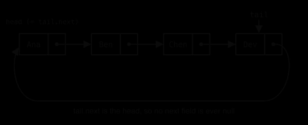
Because no pointer is ever null, a traversal cannot stop by testing for null. It stops when it arrives back at the node where it started. The loop must also run at least once, because the starting node is both where the traversal begins and the test for where it ends; this is the post-condition (do–while) pattern. Java has a do … while loop for it; Python, which has none, uses while True: with a break once the starting node comes round again.
Insertion at the end takes three steps: point the new node at the head (node.next = tail.next), point the old tail at the new node, then move tail. Deletion is the same bypass as in a singly linked list, with two extra cases: deleting the only node leaves the list empty, and deleting the tail moves tail back to the previous node. The diagram shows both operations.
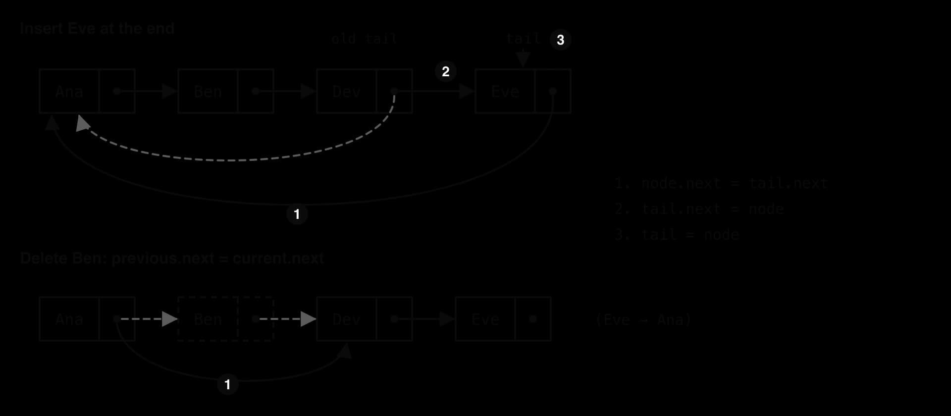
The class CircularLinkedList implements the turn order of a board game. After the players are added, a reference that keeps following next hands out turns forever, wrapping from the last player to the first with no special code.
Python
class Node:
    def __init__(self, data):
        self.data = data
        self.next = None


class CircularLinkedList:
    """Singly linked and circular: tail.next is always the first node."""

     ():
        .tail =

     ():
        node = Node(value)
         .tail  :
            node. = node
        :
            node. = .tail.
            .tail. = node
        .tail = node

     ():
         .tail  :
            ()

        current = .tail.
        text =
         :
            text = text + current.data +
            current = current.
             current  .tail.:

        (text)

     ():
         .tail  :

        previous = .tail
        current = .tail.
         :
             current.data == target:
                 current  previous:
                    .tail =
                :
                    previous. = current.
                     current  .tail:
                        .tail = previous

            previous = current
            current = current.
             current  .tail.:


players = CircularLinkedList()
 name  [, , , ]:
    players.insert_at_end(name)
players.display()

turn = players.tail.
 i  ():
    (, i + , , turn.data)
    turn = turn.

players.delete()
players.display()
players.delete()
players.display()
(, players.tail.data, , players.tail..data)
Java version
Java
class Node {
    String data;
    Node next;

    Node(String data) {
        this.data = data;
    }
}


  {
       ;

       {
            (value);
         (tail == ) {
            node.next = node;
        }  {
            node.next = tail.next;
            tail.next = node;
        }
        tail = node;
    }

       {
         (tail == ) {
            System.out.println();
            ;
        }
           tail.next;
           ;
         {
            text = text + current.data + ;
            current = current.next;
        }  (current != tail.next);
        System.out.println(text);
    }

       {
         (tail == ) {
             ;
        }
           tail;
           tail.next;
         {
             (current.data.equals(target)) {
                 (current == previous) {
                    tail = ;
                }  {
                    previous.next = current.next;
                     (current == tail) {
                        tail = previous;
                    }
                }
                 ;
            }
            previous = current;
            current = current.next;
        }  (current != tail.next);
         ;
    }
}

   {
        {
            ();
        String[] names = {, , , };
         (String name : names) {
            players.insertAtEnd(name);
        }
        players.display();

           players.tail.next;
         (   ; i < ; i++) {
            System.out.println( + (i + ) +  + turn.data);
            turn = turn.next;
        }

        players.delete();
        players.display();
        players.delete();
        players.display();
        System.out.println( + players.tail.data +  + players.tail.next.data);
    }
}
Turns 5 and 6 wrap round to Ana and Ben without any index arithmetic, and after Dev (the tail) is deleted, Ben becomes the tail and still points back to Ana.
Plain text
Ana Ben Chen Dev
Turn 1 -> Ana
Turn 2 -> Ben
Turn 3 -> Chen
Turn 4 -> Dev
Turn 5 -> Ana
Turn 6 -> Ben
Ana Ben Dev
Ana Ben
tail is Ben and tail.next is Ana
Circular lists suit any process that cycles through a fixed group repeatedly: turns in a multiplayer game, a music player's "repeat all" mode (a circular doubly linked list also gives "previous track"), slides in a looping presentation, and round robin scheduling, in which the operating system gives each ready process a time slice in turn and returns to the first process after the last (subtopic A1.3, Operating systems and control systems). A process that finishes is deleted from the loop; a new one is inserted just before the current position, so it waits a full round.
Evaluating linked lists
Linked lists and arrays both store a sequence but make opposite trade-offs. An array (including the dynamic arrays behind ArrayList and the Python list) keeps elements contiguous and calculates any address directly; a linked list scatters its nodes and finds an element only by following pointers. The Big O comparison sets out the consequences for items.
Operation | Static array | Dynamic array ( | Singly linked list (head and tail) | Doubly linked list |
|---|---|---|---|---|
Access item at index |
The Big O figures cover only running time; a full evaluation also weighs memory use and real-world speed.
Advantages of a linked list
It is a dynamic data structure: it grows one node at a time and never copies everything to a larger block, as a full dynamic array must.
Inserting or deleting at a known position changes a few pointers and shifts nothing, so the cost does not depend on the length of the list.
No memory is reserved for items that do not exist yet, whereas a static array sized for the worst case may leave most slots empty.
Disadvantages of a linked list
There is no direct access by index. Reaching item means following pointers, so code such as
for i in range(n): get(i)becomes , and binary search is impossible.Every node carries extra memory for its references. In a simplified model where a data item and a reference each take 8 bytes, 1,000 items take 8,000 bytes in an array, 16,000 bytes in a singly linked list and 24,000 bytes in a doubly linked list, before any per-object overhead the language adds.
Nodes are scattered in memory, so a traversal jumps between distant addresses. The CPU cache works best on data stored close together (subtopic A1.1), so an array is usually much faster to traverse in practice even though both are
The choice therefore depends on which operations dominate. A linked list suits data that is mostly processed in order and frequently changed at the ends or at positions the program already holds: queues, undo histories, playlists, the free-block list of a memory manager. An array or dynamic array suits data that is read by position, searched with binary search, or traversed many times, which describes most everyday collections. A doubly linked list is worth its extra pointer when the program must move backwards or delete nodes it already holds a reference to; a circular list when the program cycles through the items repeatedly.
 YouTube
Binary search trees
Trees and their vocabulary
Linked lists arrange nodes in a line, so a search may have to visit every node. A tree arranges them in branches. Each node can point to several others below it, and a search that chooses the right branch at each node skips everything in the branches it does not take. Family trees, folder structures on a disk and the organisation chart of a company all have this shape.
The tree diagram labels the parts of a tree that the rest of the topic relies on, using a tree of eight numbered nodes. By convention trees are drawn upside down, with the top node at the top of the page.
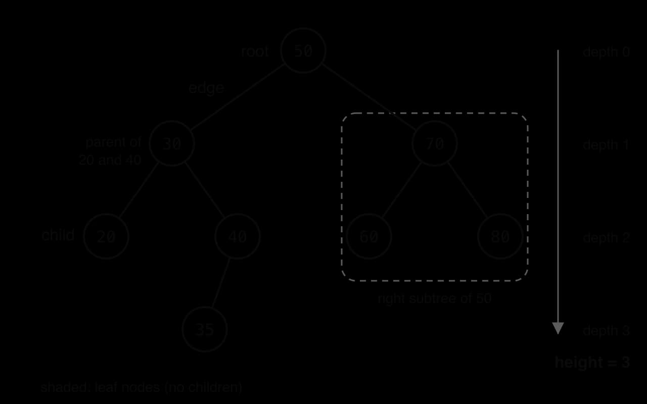
Each connection between two nodes runs from a node to one directly below it, and the vocabulary of family trees names the two ends. In the diagram, 30 is the parent of 20 and 40, and 20 and 40 are children of 30.
The relationship is relative: 30 is a child of 50 and, at the same time, the parent of 20 and 40.
Nodes at the bottom of a tree have no children. In the diagram, 20, 35, 60 and 80 are shaded to show them.
Any node, taken together with everything below it, is itself a complete tree. This property is why so many tree algorithms are recursive: an operation on a tree can be described as an operation on the root plus the same operation on each smaller tree beneath it.
The links themselves also have a name, which is used when counting the length of a path. Each node except the root has exactly one edge to its parent, so a tree of nodes always has edges.
The depth of a node is the number of edges on the path from the root to it: the root has depth 0, 30 and 70 have depth 1, and 35 has depth 3. The height of the whole tree is the greatest depth of any node.
Binary trees and the BST property
A tree in which each node has at most two children, called the left child and the right child, is a binary tree. In code, each node holds a data item and two references, left and right, either of which may be null/None. This is a linked structure like a doubly linked list, but its two references lead downwards to different subtrees instead of forwards and backwards along a line.
A binary search tree adds one rule about where values may go. For every node, all the values in its left subtree are smaller than the node's value and all the values in its right subtree are larger. The rule applies to the whole subtree, not only to the immediate children: in the example tree, 35 lies in the left subtree of 50 and in the right subtree of 30, so it must be both smaller than 50 and larger than 30.
The rule as stated leaves no place for a value equal to one already in the tree. Implementations choose a convention and keep to it: the most common is to ignore a duplicate (the tree then behaves as a set of unique keys) or to store a count in the existing node; another is to send equal values consistently to one side, for example the right. The examples that follow ignore duplicates.
Searching a BST
Searching starts at the root and makes one comparison per level. If the target equals the node's value, the search succeeds. If the target is smaller, every value in the right subtree is also too large, so the search moves to the left child; if the target is larger, it moves to the right child. Reaching an empty (null) position means the target is not in the tree.
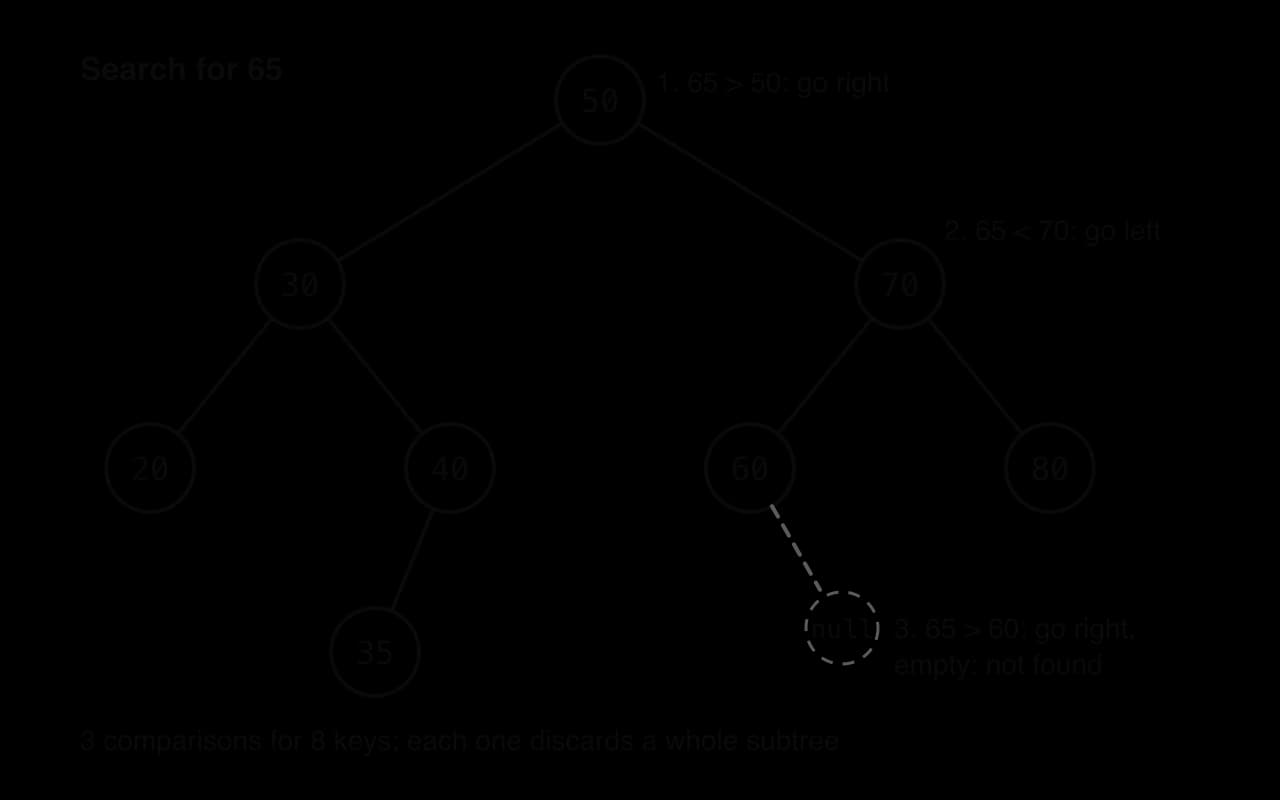
The cost of a search depends on the height of the tree, because the search follows a single path from the root downwards. In a well-shaped tree, each level holds twice as many nodes as the level above, so a tree of height holds up to nodes. Turned round, nodes need a height of only about
Inserting into a BST
Insertion follows the search path for the new value. Starting at the root, the value is compared with each node and moves left or right, exactly as a search would, until it reaches an empty position; the new node is attached there as a leaf. Existing nodes never move, so insertion changes one reference (the left or right of the last node visited) and costs the same as a search.
The insertion diagram builds a tree from the keys 50, 30, 70, 20, 40, 60, 80, 35 in that order. The first key becomes the root; every later key travels down from the root to an empty spot.

Traversing a BST
A traversal visits every node exactly once. A list has one natural order, but a binary tree offers several, depending on when a node is visited relative to its two subtrees. All three standard traversals are defined recursively, as a node plus the same traversal of its left and right subtrees, so they are examples of branching recursion (subtopic B2.4, Programming algorithms).
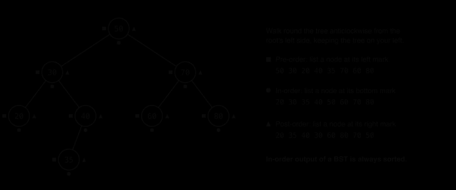
In-order is the traversal that sorts: every value in a node's left subtree is smaller and every value in its right subtree is larger, so listing left, node, right at every level produces the values from smallest to largest. Inserting keys into a BST and then traversing it in order is a complete sorting method (sometimes called tree sort).
Pre-order lists every parent before its children. Inserting the pre-order output into an empty BST rebuilds exactly the same tree shape, so pre-order is used to copy a tree or to save it to a file and load it again. It also gives the order in which a folder listing prints a folder before its contents.
Post-order lists every child before its parent. That is the safe order for deleting a whole tree (a node is removed only after everything below it) and for calculating anything that depends on the children first, such as the total size of a folder or the value of an arithmetic expression stored as a tree.
The traversal diagram gives a quick way to read all three orders off a sketch. Each node carries three marks: one on its left, one below and one on its right. A line drawn round the outside of the tree, starting at the root's left and keeping the tree on its left, passes every mark; listing each node when the line passes its left mark gives pre-order, its bottom mark in-order and its right mark post-order.
The traversals and the search take only a few lines in code, because each one is the definition written out. The listing is for reading only: BSTs are explained and sketched, not coded, but the code makes the recursive definitions concrete. Each traversal adds the node's key to the list out at a different moment.
Python
class TreeNode:
    def __init__(self, key):
        self.key = key
        self.left = None
        self.right = None


def insert(root, key):
    """Return the root of the tree after inserting key (duplicates ignored)."""
    if root is None:
        return TreeNode(key)
    if key < root.key:
        root.left = insert(root.left, key)
    elif key > root.key:
        root.right = insert(root.right, key)
    return root


def search():
    current = root
     current   :
         key == current.key:

         key < current.key:
            current = current.left
        :
            current = current.right


 ():
     node   :
        in_order(node.left, out)
        out.append(node.key)
        in_order(node.right, out)


 ():
     node   :
        out.append(node.key)
        pre_order(node.left, out)
        pre_order(node.right, out)


 ():
     node   :
        post_order(node.left, out)
        post_order(node.right, out)
        out.append(node.key)


root =
 key  [, , , , , , , ]:
    root = insert(root, key)

result = []
in_order(root, result)
(, result)
result = []
pre_order(root, result)
(, result)
result = []
post_order(root, result)
(, result)
(, search(root, ), , search(root, ))
Java version
Java
import java.util.ArrayList;

class TreeNode {
    int key;
    TreeNode left;
    TreeNode right;

    TreeNode(int key) {
        this.key = key;
    }
}

public class BstDemo {

     TreeNode  {
         (root == ) {
              (key);
        }
         (key < root.key) {
            root.left = insert(root.left, key);
        }   (key > root.key) {
            root.right = insert(root.right, key);
        }
         root;
    }

       {
           root;
         (current != ) {
             (key == current.key) {
                 ;
            }
             (key < current.key) {
                current = current.left;
            }  {
                current = current.right;
            }
        }
         ;
    }

       {
         (node != ) {
            inOrder(node.left, out);
            out.add(node.key);
            inOrder(node.right, out);
        }
    }

       {
         (node != ) {
            out.add(node.key);
            preOrder(node.left, out);
            preOrder(node.right, out);
        }
    }

       {
         (node != ) {
            postOrder(node.left, out);
            postOrder(node.right, out);
            out.add(node.key);
        }
    }

        {
           ;
        [] keys = {, , , , , , , };
         ( key : keys) {
            root = insert(root, key);
        }
        ArrayList<Integer> result =  <Integer>();
        inOrder(root, result);
        System.out.println( + result);
        result =  <Integer>();
        preOrder(root, result);
        System.out.println( + result);
        result =  <Integer>();
        postOrder(root, result);
        System.out.println( + result);
        System.out.println( + search(root, ) +  + search(root, ));
    }
}
The output matches the orders read off the diagram.
Plain text
In-order:   [20, 30, 35, 40, 50, 60, 70, 80]
Pre-order:  [50, 30, 20, 40, 35, 70, 60, 80]
Post-order: [20, 35, 40, 30, 60, 80, 70, 50]
search 60: True  search 65: False
The search uses a loop because it follows one path; the traversals use recursion because each node leads to two subtrees, both of which must be visited, and the call stack holds the return point for the subtree still to be visited. A traversal visits each of the nodes once, so it is whatever the shape of the tree.
Deleting from a BST
Removing a node must leave a tree that still obeys the BST rule. The method depends on how many children the node has, giving three cases. The deletion diagram shows each case on the same starting tree.
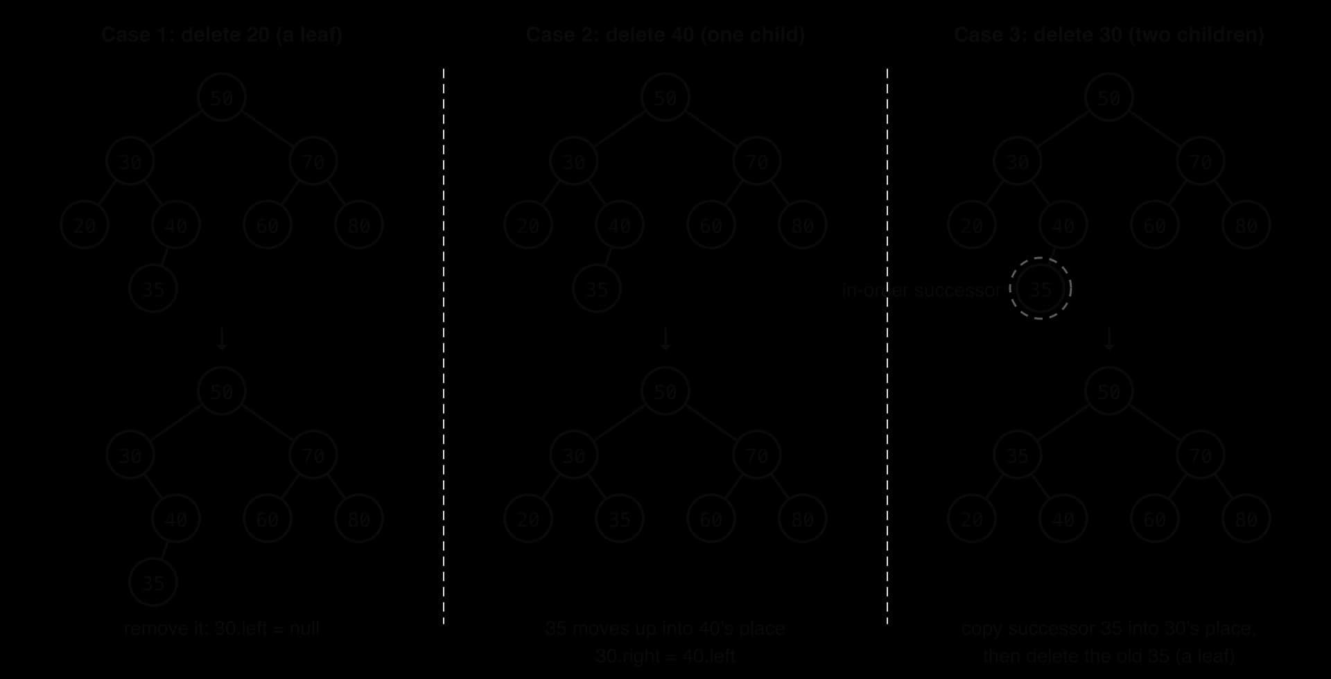
The node is a leaf. Set the parent's reference to it (
leftorright) tonull/None. Deleting 20 sets30.lefttonull.The node has one child. The child, with its whole subtree, moves up into the deleted node's place: the parent's reference is redirected to the child. Deleting 40 sets
30.rightto 35. The BST rule still holds, because everything in 40's subtree was already greater than 30.The node has two children. Neither child can simply move up, because the other subtree would have nowhere to go. Instead, the node's value is replaced by the next larger value in the tree, its in-order successor, and that successor's original node is then deleted.
To find the successor of a node with two children, move once to the right child, then keep moving left until there is no left child. For 30, the path is 30 → 40 → 35, and 35 has no left child, so 35 is the successor. Copying 35 into 30's node keeps the BST rule: 35 is larger than everything in 30's left subtree (it came from the right subtree) and smaller than everything else in the right subtree (it was the smallest there). The successor never has a left child (otherwise that child would be smaller and would be the successor), so deleting its old node is always case 1 or case 2.
Balanced and degenerate trees
The cost of a BST search depends on the tree being bushy, with levels that fill up as they go down. Nothing in the insertion method guarantees that. The shape is decided entirely by the order in which keys arrive, and the degenerate diagram shows the same seven keys inserted in two different orders.
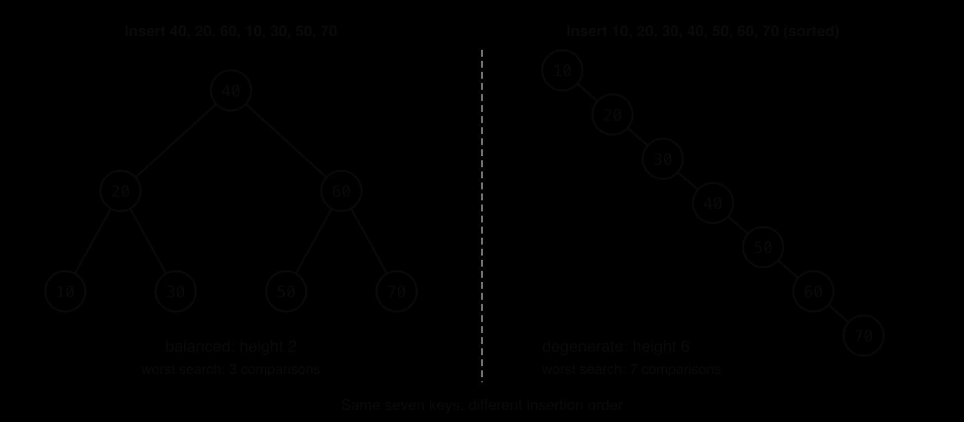
When keys arrive already sorted (or in reverse order), each new key is larger than every key so far, so it is always placed as the right child of the last one. Each node has a single child, the tree is a chain, and its height is .
The difference becomes enormous as grows. For one million keys, a balanced tree has height 19 (20 levels) while a degenerate tree has height 999,999; a search for a missing key makes at most 20 comparisons in the first and one million in the second. Most trees fall between these extremes. When keys arrive in random order, the tree is usually bushy enough that an average search makes about comparisons, so a plain BST is in the average case and
Operation | Cost in terms of height | Balanced tree, or average case (random order) | Degenerate tree (worst case) |
|---|---|---|---|
Search | |||
Insert |
Self-balancing trees solve the problem by checking the shape after each insertion or deletion and rotating nodes to restore balance, so every operation stays whatever order the data arrives in. AVL trees and red-black trees are the best-known designs; Java's TreeMap is documented as "a Red-Black tree based NavigableMap implementation".
Databases and file systems use a wider relative of the BST. A B-tree node holds many sorted keys and has many children, so the tree is very short and a lookup reads only a few blocks from the disk; each block read from secondary storage is far slower than a comparison in memory, so reducing the number of levels matters more than reducing comparisons. B-trees were invented by Rudolf Bayer and Edward McCreight at Boeing Research Labs, in a paper first circulated in July 1970, and B-tree variants sit behind most database indexes (subtopic A3.3).
When to choose a BST
A BST keeps its data in sorted order at all times, which no hash table does. That makes it the natural choice when the program needs ordered operations as well as lookups: listing items in order, finding the smallest or largest, or finding every key in a range (all orders between 9:00 and 10:00). Compared with a sorted array, a balanced BST finds items equally fast and also inserts and deletes in instead of , because no elements shift. Its costs are two references per node, more complex code, and the risk of degenerating if it is not balanced.
Sets
Characteristics of a set
Many tasks come down to membership: checking whether a username is already taken, whether a student has handed in an assignment, or which tags a post carries. A list can handle them, but a list allows duplicates and keeps an order the question does not need. A set models the mathematical idea of a collection in which each item either is or is not present.
Two properties define a set and decide how it behaves:
Unique elements. Adding an element that is already present changes nothing, so a set never holds duplicates. Converting a list to a set is the standard way to remove repeated values.
No order. A set has no first or last element and no index, so
s[0]is meaningless. Elements may come out of a loop in any order, and the order can change as the set grows.
The basic operation on a set is asking whether an element belongs to it, and the purpose of most set implementations is to make that question fast.
Set operations
Sets are combined with three operations taken from mathematics, and compared with two relations. The Venn diagrams show each one for and , with the result shaded.
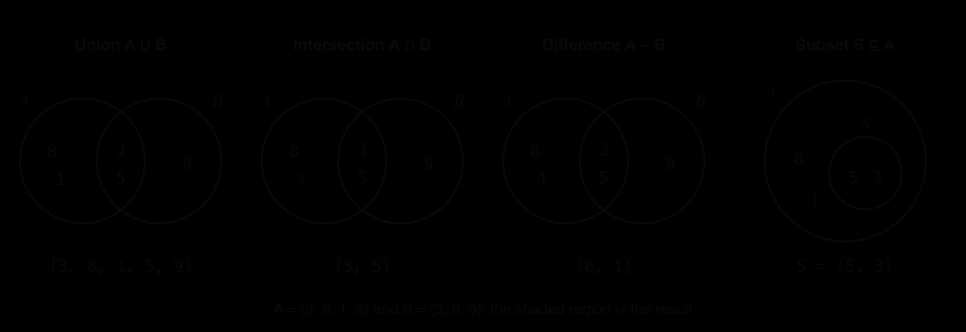
The union of and is : five elements, not seven, because 3 and 5 appear in both sets but are included once.
Only 3 and 5 belong to both sets, so . If two sets have nothing in common, their intersection is the empty set and they are called disjoint.
Difference is the only one of the three operations whose result depends on the order: , but . Union and intersection give the same result either way round.
is a subset of , because both 5 and 3 are in ; is not a subset of , because 9 is not in
Sets in Python and Java
Python and Java both provide a set built on a hash table, a structure that makes adding, removing and testing membership on average. The program records two school clubs and works out which students belong to both, to either, and to chess only.
Python
chess = {"Aiko", "Ben", "Carla", "Dmitri"}
robotics = {"Ben", "Dmitri", "Ella"}
finalists = {"Ben", "Dmitri"}

print("Ella" in robotics, "Ella" in chess)       # membership
chess.add("Ella")                                # add a new element
chess.add("Ben")                                 # already there: no change
chess.remove("Aiko")                             # KeyError if absent
chess.discard("Zara")                            # no error if absent
print(len(chess))

both = chess & robotics                          # intersection
either = chess | robotics                        # union
chess_only = chess - robotics                    # difference
print((both), (either), (chess_only))
(finalists <= robotics, robotics >= finalists)
(finalists.issubset(chess), chess.issuperset(robotics))

empty = ()
names = [, , , , ]
(((names)), )
Java version
Java
import java.util.HashSet;
import java.util.TreeSet;

public class SetsBuiltin {
    public static void main(String[] args) {
        HashSet<String> chess = new <String>();
        chess.add();
        chess.add();
        chess.add();
        chess.add();
        HashSet<String> robotics =  <String>();
        robotics.add();
        robotics.add();
        robotics.add();
        HashSet<String> finalists =  <String>();
        finalists.add();
        finalists.add();

        System.out.println(robotics.contains() +  + chess.contains());
        chess.add();
        chess.add();
        chess.remove();
        System.out.println(chess.size());


        HashSet<String> both =  <String>(chess);
        both.retainAll(robotics);
        HashSet<String> either =  <String>(chess);
        either.addAll(robotics);
        HashSet<String> chessOnly =  <String>(chess);
        chessOnly.removeAll(robotics);

        System.out.println( <String>(both) +  +  <String>(either)
                +  +  <String>(chessOnly));

        System.out.println(robotics.containsAll(finalists) +  + robotics.containsAll(finalists));
        System.out.println(chess.containsAll(finalists) +  + chess.containsAll(robotics));

        String[] names = {, , , , };
        HashSet<String> unique =  <String>();
         (String name : names) {
            unique.add(name);
        }
        System.out.println(unique.size() + );
    }
}
Both versions print the same results (Java writes true, false and [Ben, Dmitri, Ella] in its own style):
Plain text
True False
4
['Ben', 'Dmitri', 'Ella'] ['Ben', 'Carla', 'Dmitri', 'Ella'] ['Carla']
True True
True True
3 different names
The results are printed through sorted() (Python) and TreeSet (Java) only so that the output is predictable; the sets themselves have no order. The operations map between the languages as follows.
Operation | Python | Java |
|---|---|---|
Create empty |
|
|
Membership |
|
|
Add |
|
|
Remove |
|
|
Size |
|
|
Union |
|
|
Intersection |
|
|
Difference |
|
|
Subset |
Python has its own trap with empty sets. Curly braces with elements, {"Ben", "Ella"}, make a set, but empty curly braces, {}, make an empty dictionary, so an empty set must be written set(). Python sets also accept only hashable (in practice, immutable) elements: numbers, strings and tuples can be stored, but a list cannot, for reasons that follow from how hash tables work.
Sets without built-in methods
Where the built-in set type or its methods cannot be used, the operations are written by hand, usually with a list or array holding the elements. The class ListSet implements the set ADT on top of a plain list. Membership is a linear search; add checks membership first so that duplicates never enter; remove fills the gap with the last element, which is allowed because a set has no order. Union, intersection, difference and subset are loops over one set that test membership in the other.
Python
class ListSet:
    """Set ADT stored in a plain list, written without set built-ins."""

    def __init__(self):
        self.items = []

    def contains(self, value):            # membership: linear search
        for item in self.items:
             item == value:


     ():
          .contains(value):
            .items.append(value)

     ():
         i  ((.items)):
             .items[i] == value:
                .items[i] = .items[(.items) - ]
                .items.pop()


     ():
        result = ListSet()
         item  .items:
            result.add(item)
         item  other.items:
            result.add(item)
         result

     ():
        result = ListSet()
         item  .items:
             other.contains(item):
                result.add(item)
         result

     ():
        result = ListSet()
         item  .items:
              other.contains(item):
                result.add(item)
         result

     ():
         item  .items:
              other.contains(item):


     ():
         other.is_subset()


a = ListSet()
b = ListSet()
 value  [, , , , ]:
    a.add(value)
 value  [, , ]:
    b.add(value)
(, a.items, , b.items)
(, a.union(b).items)
(, a.intersection(b).items)
(, a.difference(b).items)
small = ListSet()
small.add()
small.add()
(small.is_subset(a), a.is_superset(small), b.is_subset(a))
a.remove()
(, a.items)
Java version
Java
The second 8 is ignored when a is built, so a has four elements. After remove(3), the last element (5) has moved into the gap at the front, which is harmless for a set.
Plain text
a = [3, 8, 1, 5]  b = [5, 9, 3]
union        [3, 8, 1, 5, 9]
intersection [3, 5]
a - b        [8, 1]
True True False
after remove(3): [5, 8, 1]
The hand-written version shows why built-in sets use hash tables. Every contains call scans the list, , and union, intersection, difference and subset call contains once for each element of the other set, so for sets of sizes and they cost . With a hash-based set, each membership test is
Operation | List-based set (by hand) | Hash-based set ( |
|---|---|---|
Membership, add, remove | average, worst | |
Union, intersection, difference |
Sets appear wherever a program needs uniqueness or overlap rather than order: removing duplicate email addresses before a mailing, finding the friends two users have in common (an intersection), suggesting people a user might know (friends of friends minus existing friends, a difference), checking that a user holds every permission a page requires (a subset test), and recording which words a spell checker knows.
Hash tables
Maps and key–value pairs
A set records only whether each item is present. Many programs need a second piece of information with each item: the price of a product code, the phone number for a name, the count of each word in a text. The map ADT stores exactly that.
In a phone book, each name is a key and each phone number a value. Keys must be unique, because the key identifies the entry; values may repeat, since two people can share a number.
A set can be seen as a map that stores keys and no values, and both are usually built on the same structure: the hash table. Its aim is to find an item by its key in time on average, without searching. A sorted array with binary search needs and a list needs ; a hash table instead calculates where the item must be.
How a hash table works
A hash table is an array of positions called buckets. To store a key, a hash function converts the key into a number, and that number, reduced to the range of valid indices, says which bucket to use. To find the key later, the program runs the same function on it and goes straight to the same bucket, without examining any other.
The calculation is done by a function that must always give the same answer for the same key.
The number the hash function produces is reduced to a valid index with modulo: for a table of buckets, the index is the hash value mod , which is always between 0 and . For integer keys, the key itself can serve as the hash value, so
The array position selected in this way is called a bucket, because in many designs it can hold more than one key.
With 4 buckets, "pen" goes to bucket 3. "ink" gives , and "map" gives
A good hash function for a hash table has four properties:
Deterministic: the same key always gives the same hash value, otherwise a stored key could never be found again.
Fast: it is calculated on every insertion and lookup, so it must take time (or time proportional to the key's length for strings).
Uniform: it spreads keys evenly across all buckets, so that no bucket collects far more keys than the others.
Uses the whole key: every part of the key affects the result. Summing character codes fails this test in a subtle way: anagrams such as "listen" and "silent" always collide, because addition ignores the order of the letters. Java's
String.hashCode()instead multiplies by 31 at each step,
Collisions
Collisions cannot be avoided. A hash function maps a very large set of possible keys (every possible string, for instance) onto a small number of buckets, so by the pigeonhole principle many keys must share each index. Even with far fewer keys than buckets, collisions come early: with 365 buckets and random hash values, 23 keys are enough for a collision to be more likely than not, the same mathematics as the "birthday problem".
A collision resolution strategy decides where the second key goes and how lookups still find it. The two families are separate chaining and open addressing.
The chaining diagram stores the integer keys 15, 22, 8, 31 and 12 in a table of 7 buckets using . Three keys hash to bucket 1, so bucket 1 holds a chain of three nodes; each new key is added at the front of its chain, which is an linked-list insertion.
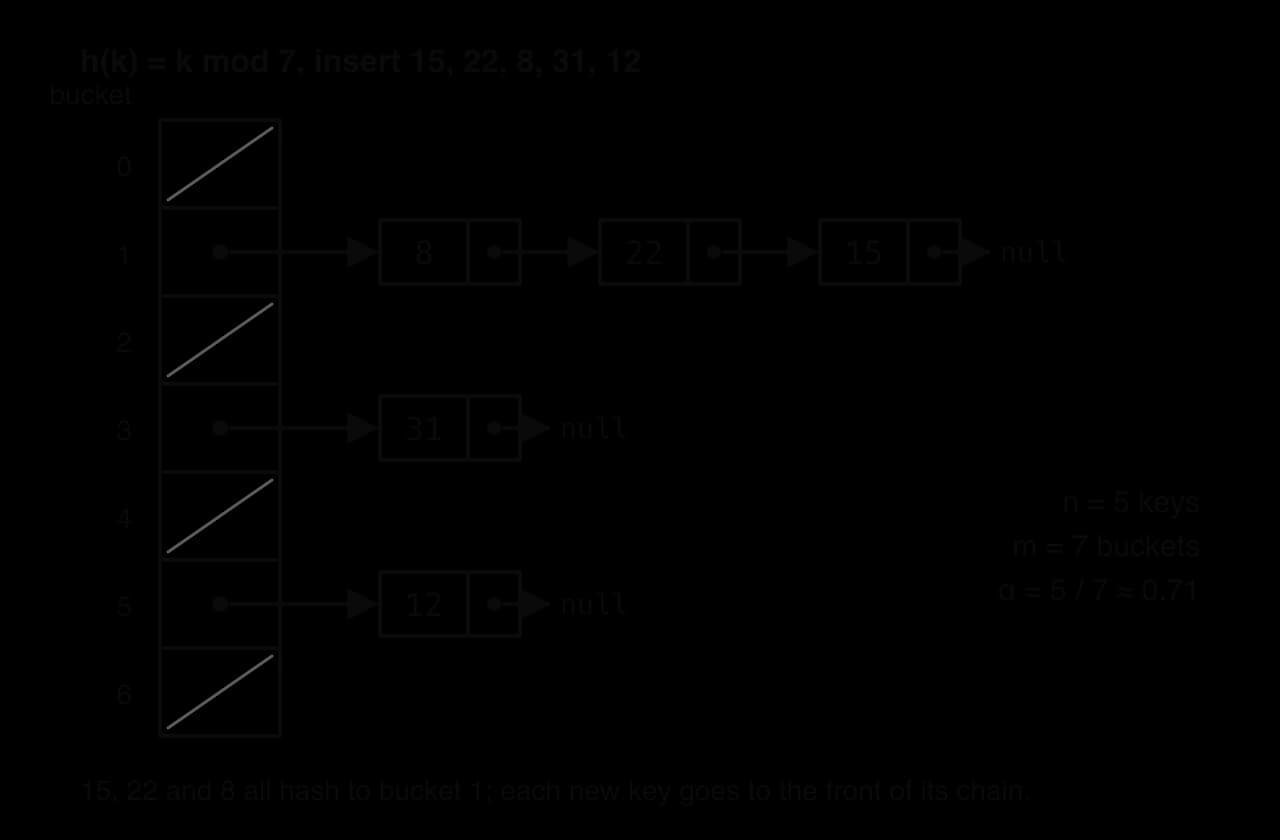
To look up a key, the program hashes it to find the bucket, then searches that bucket's chain. To delete a key, it is removed from its chain like any linked-list node. Chaining never runs out of room, because chains can grow, and its performance falls gradually as the table fills.
The simplest probe sequence tries the next bucket along, and the next, wrapping round from the last index to index 0.
The probing diagram stores the same five keys in a table of 7 slots with linear probing. 15 goes to its home slot, 1. 22 also hashes to 1, finds it taken and moves to 2. 8 hashes to 1 as well and has to step past 1 and 2 to reach 3. 31 hashes to 3, which 8 has now taken, so it moves to 4, even though no key with home 3 had been inserted before. 12 goes straight to its home slot, 5.
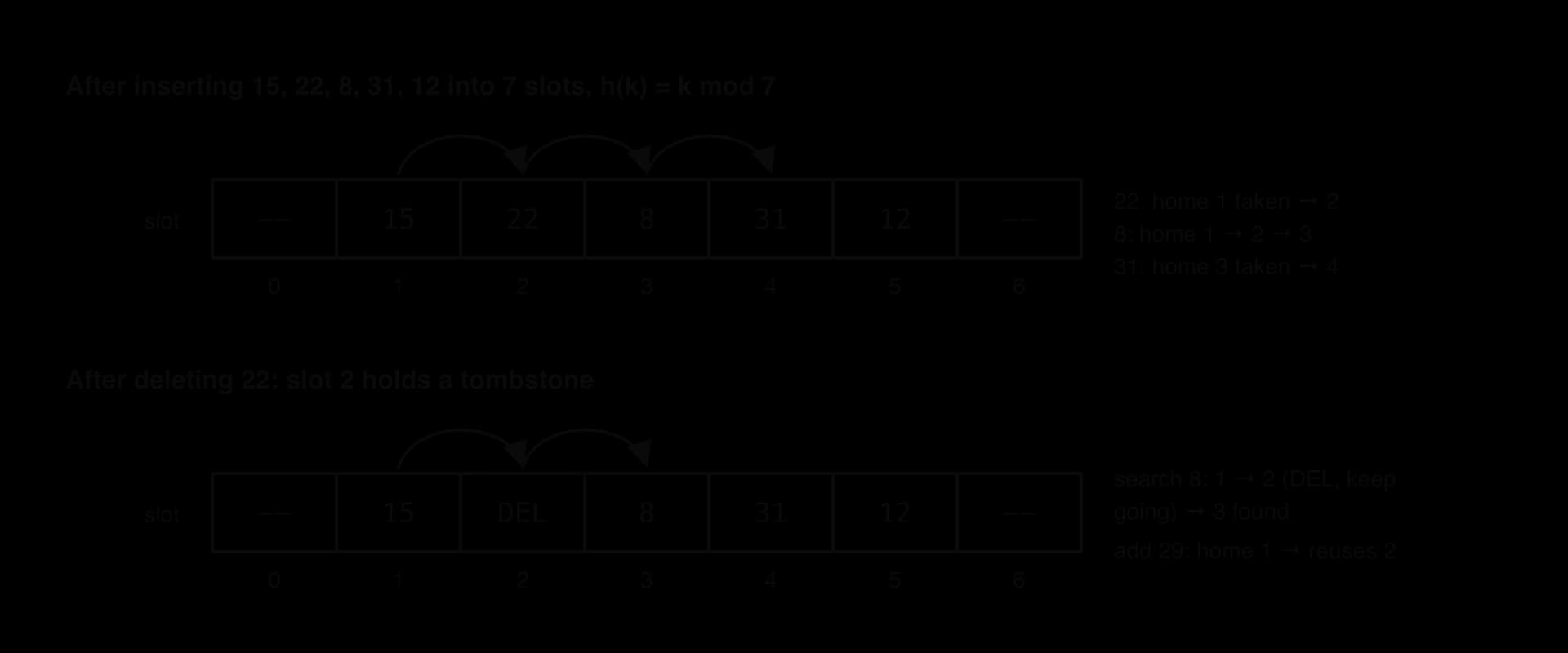
A search with linear probing follows the same sequence as insertion: start at the home slot and step forward until the key is found or an empty slot is reached. An empty slot proves the key is absent, because an insertion would have used it. Linear probing keeps all data in one array, which uses memory efficiently and is fast for the CPU cache, but it suffers from clustering: occupied slots join into long runs, any key that hashes anywhere into a run must walk to its end, and the run grows longer still.
Deletion in open addressing cannot simply empty a slot. If 22 were removed by marking slot 2 empty, a later search for 8 would start at slot 1, find 15, move to slot 2, find it empty and wrongly report that 8 is absent, although 8 is in slot 3. The fix is to mark the slot with a special value.
Search and insertion treat a tombstone differently. A search treats a tombstone as occupied and keeps probing, stopping only at the key or at a truly empty slot. An insertion first searches for the key, so that no duplicate is added, and then places it in the first empty slot or tombstone along its probe sequence. In the probing diagram, after 22 is deleted, a search for 8 passes the tombstone in slot 2 and finds 8 in slot 3; adding 29 (home slot 1) then reuses slot 2. A table that accumulates many tombstones gets slower, because searches must step over them, so implementations clear them out when the table is rehashed.
Load factor and rehashing
How full a hash table is decides how often collisions happen and how long chains or probe sequences become. The measure of fullness is the load factor.
With separate chaining, the load factor is the average length of a chain, so an unsuccessful search examines about entries after hashing, and a successful one about . The load factor can exceed 1 (there can be more entries than buckets), with performance falling gradually. With open addressing, the load factor can never exceed 1, and performance collapses as it approaches 1, because clusters merge into ever longer runs. The graph plots the expected number of slots examined for linear probing against the load factor, using Knuth's standard approximations.
Source: approximations from D. E. Knuth, The Art of Computer Programming, Volume 3: Sorting and Searching, 2nd edition (Addison-Wesley, 1998), section 6.4, Hashing: linear probing ≈ ½(1 + 1/(1 − α)²) slots for an unsuccessful search and ½(1 + 1/(1 − α)) for a successful one; separate chaining ≈ 1 + α/2 for a successful search. They assume random hash values and a large table.
The cure for a high load factor is to make the table bigger. Because every index is calculated modulo the table size, keys cannot simply be copied across to a larger array: each one must be hashed again with the new size.
A rehash costs , because every entry is moved. It happens rarely, though: after doubling, the table must take as many new entries again before the next rehash, so the total cost spread over all insertions is still per insertion on average, the same argument that makes appending to a dynamic array cheap (subtopic B2.2). The trade-off is between time and space: a low threshold keeps chains short but leaves many buckets empty; a high threshold saves memory but makes every operation slower.
In most chained tables, including Java's HashMap, each bucket's chain is a singly linked list. Adding a key means searching its chain first, so that an existing key is updated instead of duplicated, then linking in a new node (at the front in the worked example; Java's HashMap adds it at the end); removing a key is a linked-list deletion that bypasses one node.
Big O of hash table operations
With a reasonable hash function and the load factor kept below a fixed threshold, the expected number of entries examined does not grow with , so insertion, lookup and deletion are in the average case. In the worst case, if every key hashes to the same bucket, the table becomes a single chain (or a single cluster), and every operation is , no better than a list.
Operation | Average case | Worst case | Cause of the worst case |
|---|---|---|---|
Insert (put, add) | all keys in one bucket; or a rehash | ||
Lookup (get, contains) |
The worst case can also be caused deliberately. An attacker who knows a server's hash function can send thousands of keys chosen to collide, making each request and slowing the server down; this is a form of denial of service. Python reduces this risk by default: the documentation explains that the hash values of str and bytes objects are "salted" with an unpredictable random value that is constant within one run of Python but different between runs. Java's HashMap limits the damage differently, as the case study shows.
HashMap and dict, HashSet and set
Java and Python both provide hash-table maps and sets, and programs use these rather than writing their own. The program counts how often each word appears in a short text, the standard use of a map.
Python
words = "the cat and the dog and the bird".split()

counts = {}                                   # empty dict
for word in words:
    counts[word] = counts.get(word, 0) + 1    # 0 if the key is absent
print(counts)

print("cat" in counts, "fish" in counts)      # key lookup, average O(1)
print(counts["the"], counts.get("fish", 0))
del counts["dog"]                             # remove a key-value pair
for word in counts:                           # keys come out in insertion order
    print(word, counts[word])
Java version
Java
import java.util.HashMap;

public class MapsDemo {
    public static void main(String[] args) {
        String[] words = "the cat and the dog and the bird".split(" ");

        HashMap<String, Integer> counts = new HashMap<String, Integer>();
        for (String word : words) {
            counts.put(word, counts.getOrDefault(word, 0) + 1);   // 0 if the key is absent
        }
        System.out.println(counts);

        System.out.println(counts.containsKey("cat") + " " + counts.containsKey("fish"));
        System.out.println(counts.get("the") + " " + counts.getOrDefault("fish", 0));   // get() gives null if absent
        counts.remove("dog");                                     // remove a key-value pair
        for (String word : counts.keySet()) {
            System.out.println(word +  + counts.get(word));
        }
    }
}
The Python version prints the keys in the order they were first added; the Java version prints them in an order decided by their hash codes (the, and, cat, bird on one run), and writes the map as {the=3, and=2, ...}.
Plain text
{'the': 3, 'cat': 1, 'and': 2, 'dog': 1, 'bird': 1}
True False
3 0
the 3
cat 1
and 2
bird 1
Operation | Python | Java |
|---|---|---|
Create empty |
|
|
Add or update |
|
|
Get (key must exist) |
|
|
Get with a default |
|
|
Key present? |
|
|
Remove |
|
|
Loop over keys |
|
|
Number of pairs |
|
|
The implementations behind these classes differ in ways that explain their behaviour.
Java's HashMap uses separate chaining: each bucket holds a chain of nodes.
HashSetis, in its documentation's words, "backed by a hash table (actually a HashMap instance)": it stores each element as a key of an internalHashMapand ignores the value. Neither guarantees any iteration order.Python's dict and set use open addressing in a single table, with a pseudo-random probe sequence that avoids clustering (sets first try a few neighbouring slots). The CPython source resizes a dict when it is two-thirds full. Since Python 3.7, a
dictis guaranteed to keep keys in insertion order; asetis described as an "unordered collection of distinct hashable objects" and keeps no order.
Keys must keep the same hash value for as long as they are stored. If a key changed after insertion, its hash would point to a different bucket, and the entry would be lost in the wrong place. Python therefore accepts only hashable objects (immutable ones such as numbers, strings and tuples of them) as dict keys and set elements; {[1, 2]} raises a TypeError. Java allows any object as a key but relies on its hashCode() and equals() methods agreeing: two objects that are equals must return the same hashCode(), and a key object must not be changed while it is in the map.
 YouTube
Case study: Java's HashMap
Java's HashMap is one of the most heavily used hash tables in the world, and its design shows hashing, chaining, load factors, rehashing and balanced trees combined in one real engineering trade-off. Its default settings, its resize rule and the reasons behind them are set out in its documentation and in the comments of its source code.
Defaults and resizing. A HashMap created with new HashMap<>() starts with 16 buckets and a load factor threshold of 0.75. The documentation states that when the number of entries "exceeds the product of the load factor and the current capacity", the table is rehashed "so that the hash table has approximately twice the number of buckets", and that 0.75 "offers a good tradeoff between time and space costs". The table sizes and thresholds therefore follow a fixed pattern.
Buckets (capacity) | Threshold = capacity × 0.75 | Rehash happens when inserting entry number |
|---|---|---|
16 | 12 | 13 |
32 | 24 | 25 |
64 | 48 | 49 |
128 | 96 | 97 |
Source: Oracle, Java SE 21 API documentation for HashMap (default capacity 16, load factor 0.75, rehash to about twice the buckets); OpenJDK source file HashMap.java (resize when the size exceeds the threshold; new capacity = old capacity × 2).
Choosing a bucket. Capacities are always powers of 2, so instead of hash % capacity the source uses the faster bitwise (capacity - 1) & hash, which keeps the lowest bits of the hash. Because only the low bits are used, the source first mixes the high bits of hashCode() into the low ones with h ^ (h >>> 16). For the key "pen", String.hashCode() gives ; after mixing, 110,872; and with 16 buckets,
How long chains really get. The source code's comments calculate how chain lengths are distributed when hash codes are random and the table is resized at a load factor of 0.75. Most buckets are empty or hold one entry, and long chains are vanishingly rare.
Entries in a bucket | Expected fraction of buckets | About 1 bucket in |
|---|---|---|
0 | 0.607 | 1.6 |
1 | 0.303 | 3.3 |
2 | 0.0758 | 13 |
3 | 0.0126 | 79 |
4 | 0.00158 | 633 |
5 | 0.00015795 | 6,331 |
6 | 0.00001316 | 75,988 |
7 | 0.00000094 | 1,063,830 |
8 | 0.00000006 | 16,666,667 |
Source: comments in the OpenJDK source file java/util/HashMap.java (Poisson distribution with parameter about 0.5), retrieved October 2026; the last column is 1 ÷ the fraction.
Defending the worst case. Chains are linked lists, so a bucket that receives many keys, through a poor hashCode() or a deliberate attack, makes lookups . Since Java 8 (JDK Enhancement Proposal 180, which aimed to "improve the performance of java.util.HashMap under high hash-collision conditions by using balanced trees rather than linked lists"), a bucket that already holds 8 entries (TREEIFY_THRESHOLD = 8) is converted into a red-black tree, a balanced BST, when another entry is added to it, provided the table has at least 64 buckets; it turns back into a list when it shrinks to 6 entries. The source comments explain that tree nodes are "about twice the size of regular nodes", so trees are used only where they pay for themselves, and give the result: "worst-case O(log n)" lookups in a crowded bucket instead of .
Evaluation. The design combines three structures. An array gives access to a bucket; a linked list holds the few entries a bucket normally has with almost no overhead; a balanced BST takes over only in the rare crowded bucket, capping the worst case. The 0.75 threshold spends memory (at least a quarter of the buckets are always empty) to keep chains short, and doubling makes rehashes rare enough that insertion stays on average. The limitations remain those of every hash table: no ordering of keys, an occasional pause when a large map rehashes, and dependence on key classes implementing hashCode() and equals() correctly. A program that needs keys in order uses TreeMap instead, accepting
Choosing an ADT
Arrays, linked lists, stacks, queues, trees and hash tables each make some operations cheap and others expensive. Choosing one starts from the operations the problem performs most often, then compares their cost in each candidate structure.
Structure | Access by position | Search by value | Insert / delete | Keeps order | Main strength |
|---|---|---|---|---|---|
Array or dynamic array | ; if sorted |
Exam focus
Fundamentals of ADTs is HL only and is examined on Paper 2, in questions that you answer in the language you studied (Python or Java). The statements use several command terms, and each asks for something different:
Explain (the purpose of ADTs, BSTs, hash table mechanics): a point plus its reason or consequence, for example how a collision is resolved and why the search still works.
Sketch (linked lists, BSTs): a labelled diagram showing nodes, pointers,
nulland head/tail; marks go to correct structure and links, not neatness.Construct (linked lists, sets): working code. Marks are given for features such as handling the empty list, updating pointers in a safe order, correct loop termination and the return value; minor syntax slips are usually not penalised, but a wrong pointer is.
Evaluate (linked lists): strengths and limitations tied to the scenario, ending in a judgement.
Trace (hash tables, traversals): every step recorded in order, not only the final state.
Typical question shapes (inferred from earlier IB Computer Science papers, not from official 2027 material) include: sketching a linked list after a sequence of insertions and deletions (3–4 marks); writing a method to delete a node with a given value (5–6 marks); sketching the BST formed from a list of keys and stating its traversals (3–5 marks); explaining how a node with two children is deleted (3 marks); writing code for a set operation, sometimes without built-in methods (3–4 marks); and tracing insertions into a small hash table with a given hash function and collision strategy (3–4 marks).
The markscheme answer for (d) follows the hash calculations , ,
When a question asks for code "without using built-in functions", write the loops yourself: linear search for membership, a loop with a counter instead of len, and nested loops for set operations. Using a banned built-in earns no credit for that part, even if the result is correct.
Practice questions
Define the term abstract data type. [2]
Outline two differences between a singly linked list and a doubly linked list. [4]
A circular singly linked list is accessed only through a
tailreference. Explain how the program can reach the first node, and why a traversal must not stop when it meetsnull. [3]Sketch the BST formed by inserting 60, 25, 80, 10, 40, 70, 90, 35, 45 in that order, and state its post-order traversal. [4]
Using the tree from question 4, explain how the node 25 is deleted, and sketch the resulting tree. [4]
Explain why inserting keys into a BST in ascending order makes searching inefficient, and state the Big O of a search in that case. [3]
Construct a function
is_subset(a, b)that returnsTrueif every element of listais also in listb, without using built-in set types or theinoperator. [4]A hash table of 10 slots uses
Answers
A description of a data type by the values it can hold and the operations that can be performed on it [1], without specifying how the data is stored or how the operations are implemented [1].
Any two, [2] each: each node of a doubly linked list has a
prevreference as well asnext, so it uses more memory per node; a doubly linked list can be traversed backwards as well as forwards; deleting a node given a reference to it is in a doubly linked list because its predecessor is known, whereas a singly linked list must traverse from the head to find the predecessor; insertion and deletion in a doubly linked list update four or two pointers rather than two or one.The first node is
tail.next[1]. The last node points back to the first, so no reference in the list is evernull[1]; a loop that waits fornullnever ends, so the traversal stops when it returns to the starting node [1].Tree: 60 root; 25 left, 80 right; 10 and 40 children of 25; 70 and 90 children of 80; 35 and 45 children of 40 [2]. Post-order: 10, 35, 45, 40, 25, 70, 90, 80, 60 [2].
25 has two children [1]. Its in-order successor is found by going right to 40 then left to 35, the smallest value in its right subtree [1]. 35 is copied into 25's node [1] and the old 35 leaf is removed (
40.left = null) [1]. Result: 60; 35, 80; 10, 40 (40 has right child 45); 70, 90.Each new key is larger than all previous keys, so it becomes the right child of the last node inserted [1]; the tree degenerates into a chain of height
Summary
An abstract data type is defined by its values and operations, not by its implementation; one ADT (a stack, queue, list, set or map) can be implemented in several ways, and code that uses only the operations works with any of them.
A linked list stores items in nodes that hold data and a pointer to the next node, reached from a head pointer and ended by
null/None; a doubly linked list addsprevpointers, and a circular list links the last node back to the first.Inserting at the head or tail and deleting at a known node are in a linked list, but access by position and search are , binary search is impossible, and every node costs extra memory; pointer changes must be made in an order that never loses the rest of the list.
A BST keeps every left-subtree value smaller and every right-subtree value larger than the node; search, insertion and deletion follow one path from the root,
Self-check
- To do:
I can explain the difference between an ADT and its implementation, using a stack implemented by an array and by a linked list.
- To do:
I can give four reasons for designing a collection as an ADT.
- To do:
I can sketch singly, doubly and circular linked lists with head, tail and
nulllabelled. - To do:
I can show, with numbered steps, the pointer changes for inserting at the head, inserting after a node and deleting a node, in an order that never loses part of the list.
- To do:
I can write code to traverse, search, insert into and delete from a linked list, including the empty-list and head cases.
- To do:
I can traverse a circular linked list without an infinite loop.
- To do:
I can evaluate a linked list against an array for a given scenario, using Big O, memory and cache behaviour.
- To do:
I can sketch the BST produced by a sequence of insertions and state its height.
- To do:
I can write out the in-order, pre-order and post-order traversals of a binary tree and say what each is used for.
- To do:
I can delete a leaf, a node with one child and a node with two children from a BST, finding the in-order successor correctly.
- To do:
I can explain why a BST built from sorted data has